Mayfield. HYPOTHESIS 1: Boys at Mayfield School are Taller and Weigh more on average in comparison to females HYPOTHESIS 2: Key stage 4 students who watch more hours of television on average have a lower IQ Level
Mayfield School Coursework
Introduction
I have been set to complete a statistical investigation around the fictitious data of Mayfield High School, which has data of a real school. I will therefore be completing this investigation for the subject mathematics - statistics. I will be using various techniques that I have recently studied, learnt and captured to produce a successful & efficient coursework. Alternate Statistical Methods will be used throughout this assignment to prove if my hypothesis is either correct or incorrect.
Task/Situation
I have decided to investigate majorly between the relationships the height and weight of the pupils and to tell whether or not there is any correlation between them. I will take many actions as possible in achieving pure and efficient results to meet the needs and requirement of my assignment. To meet my particular aim I will use many statistical interpretations and methods to help me form sufficient conclusions on what I have gained and obtained from the evidence that I will be collecting for this project.
My Hypothesis
A hypothesis is the outline of the idea/ideas which I will be testing and below are the following hypothesis I have decided to investigate for this particular assignment:
HYPOTHESIS 1: 'Boys at Mayfield School are Taller and Weigh more on average in comparison to females'
HYPOTHESIS 2: 'Key stage 4 students who watch more hours of television on average have a lower IQ Level'
I will now investigate the correlation between the hypothesis that I have decided to investigate and proceed with a full investigation.
HYPOTHESIS 1: 'Boys at Mayfield School are Taller and Weigh more on average in comparison to females'
Planning
I will need the data of Mayfield High School between the Years of 7 to 11 and this is due to the fact for a wider sampling range, my hypothesis is a generalization and sufficient and unbiased results. The total number of students in the school is 1183. I have used two way tables to differentiate the amount of males and females in each year (App. 1). I did this so I could take a sample as it would then be easier to works with.
I will use Stratified Sampling (App. 2) to investigate my First Hypothesis. This is because it took into thought all our needs of the sampling of the data; and this methods was easily accessible and can be easily manipulated and carried and only asked for a simple understanding of the subject.
The variables for the sample are gender and age so I had to do separate samples for boys and girls and vary the amount of samples taken from each year to keep the sample unbiased and insufficient. This was done as the different year groups had different numbers of pupils and it would be unfair to take the same number of samples from each year group i.e. 5 samples out of 55 is be more than 5 samples out of 200 so stratified sampling will be helpful this is due to the fact the number of student in each year and so there is less chance of unequal representation. I will be investigating 20 boys and Girls from each Year altogether.
I will be calculating my Stratified Sampling using the Table (App.2) and I will need calculation proportion to stratify my data spread/range.
Tally and Frequency Chart
Now that I have my data I will put them into frequency/tally tables to make it easier to read and it is a useful way of representing and helps view trends within my sampling that I have produced:
) Boys Heights
BOYS
Height (cm)
Tally
Frequency
30?h<140
II
2
40?h<150
0
50?h<160
IIIIII
6
60?h<170
IIIIIIII
8
70?h<180
I
80?h<190
III
3
90?h<200
0
A Pattern I have spotted in this particular Frequency/Tally table is that nearly 75 percent of boys are of the height between 150 to 170 from my sample and this shows me that students in my sample are rather tall and a steady size or above for their age group
2) Boys Weights
BOYS
Weight (kg)
Tally
Frequency
30?w<40
IIII
4
40?w<50
IIIIIII
7
50?w<60
IIIIII
6
60?w<70
III
3
70?w<80
0
0
This Tally and Frequency table shows the boy's weight and the spread of data are large and not as compact as the height whereas the height are rather scattered and vary. This however notifies me that some of the students in my sample and tall for their age but weight are average in relationship to their height.
Girls Heights
Tally and Frequency charts are regularly used to process raw data making easier to spot irregularities and patterns.
GIRLS
Height (cm)
Tally
Frequency
30?h<140
0
40?h<150
IIIII
5
50?h<160
IIIIIIIII
9
60?h<170
IIII
4
70?h<180
II
2
80?h<190
0
This table shows me nearly 50 percent of students are between the height of 150-160 and there are not many student who excel over 180 cm tall which and there are also not many if any student with a height between 130 to 140 cm which shows me that the spread of data is compact which makes it easier to view trends and also it shows that there are not many irregularities in height in the student in my sample that I have taken.
Girls Weight
GIRLS
Weight (kg)
Tally
Frequency
30?w<40
IIIII
5
40?w<50
IIIIIIII
8
50?w<60
IIIIII
6
60?w<70
I
70?w<80
0
Comparisons of Tally & Frequency Table
I will now compare each of the tables of girls & boys height and then weight and view the differences in trends and if there are and mistakes or bias.
Height Comparison: From the Sample I have taken I have come to find that boys grow rapidly at a later age whereas girls grow faster from an earlier age and stop at a particular age also. This is shown since I have found that 2 students are of a height between 130- 139 cm, which shows that my data may be misleading or there is a lapse in growth. Both Girls and Boys have average heights and are fairly balanced and of equal size. Although my Sample shows that boys on some occasion grow to above average height such as over 180 cm whereas in Girls this is rare and unique.
Weight Comparison: Most Boys and Girls weigh in the region of 40- 60 from my sample and I have found that not many girls are over the weight of 60 whereas in Males usually are borderline 60 or above when they come to the age of 16.
Mean and Mode of Frequency Data
I will now find the Mean, Median and Mode of the Frequency that I have found and this will be quick efficient and reliable and will help me gain evidence on whether boys are taller and weigh more in comparison to girls.
Mean of Girls and Boys Weight
BOYS
Weight (kg)
Tally
Frequency (f)
Mid-point (x)
fx
30?w<40
IIII
4
35
40
40?w<50
IIIIIII
7
45
315
50?w<60
IIIIII
6
55
330
60?w<70
III
3
65
95
70?w<80
0
75
0
TOTAL
20
980
Mean = Total Frequency Times Midpoint Divided by Total Frequency
980 Divided by 20 = 49 kg for BOYS
...
This is a preview of the whole essay
Mean of Girls and Boys Weight
BOYS
Weight (kg)
Tally
Frequency (f)
Mid-point (x)
fx
30?w<40
IIII
4
35
40
40?w<50
IIIIIII
7
45
315
50?w<60
IIIIII
6
55
330
60?w<70
III
3
65
95
70?w<80
0
75
0
TOTAL
20
980
Mean = Total Frequency Times Midpoint Divided by Total Frequency
980 Divided by 20 = 49 kg for BOYS
GIRLS
Weight (kg)
Tally
Frequency
(f)
Mid-point(x)
fx
30?w<40
IIIII
5
35
40
40?w<50
IIIIIIII
8
45
360
50?w<60
IIIIII
6
55
330
60?w<70
I
65
65
70?w<80
0
75
0
TOTAL
20
895
Mean = 895 divided by 20 = 44.75 rounded off to 45 kg for GIRLS
Mean of Boys and Girls Height
BOYS
Height (cm)
Tally
Frequency
Mid-point
Fx
30?h<140
II
2
35
270
40?h<150
0
45
0
50?h<160
IIIIII
6
55
930
60?h<170
IIIIIIII
8
65
320
70?h<180
I
75
75
80?h<190
III
3
85
555
90?h<200
0
95
0
TOTAL
20
3250
Mean= 3250 Divided by 20 = 162.5 = 163 cm = 1.63m
GIRLS
Height (cm)
Tally
Frequency
Mid-point
Fx
30?h<140
0
35
0
40?h<150
IIIII
5
45
725
50?h<160
IIIIIIIII
9
55
395
60?h<170
IIII
4
65
660
70?h<180
II
2
75
350
80?h<190
0
85
0
TOTAL
20
3130
Mean: 3130 Divided by 20 = 156.5 which is 157 cm = 1.57m
Comparison of Mean of Girls & Boys (Height and Weight)
In comparison of the mean I have found for both boys and girls heights the differences vary. This shows that on average from my sample boys are weigh more then the girls in my data although it may not be by a large amount. Boys from my Stratified Sample also on average are 6 cm taller than Girls.
Mode of Girls and Boys Weight
The arithmetic mean of a group of numbers is found by dividing their sum by the number of members in the group; e.g., the sum of the seven numbers 4, 5, 6, 9, 13, 14, and 19 is 70 so their mean is 70 divided by 7, or 10. Less often used is the geometric mean (for two quantities, the square root of their product; for n quantities, the nth root of their product).
Modal Weight Stem and Leaf Diagram
Boys weight
Stem
Leaf
Frequency
3
4 5 2 8
4
4
3 0 9 1 5 6 7
7
5
6 0 3 9 7 1
6
6
4 0 2
3
7
0
8
0
Key 3 / 4 = 34 kg
Girls weight
Stem
Leaf
Frequency
3
0 7 6 6 8
5
4
0 1 7 0 7 0 6 5
8
5
2 2 7 2 6 9
6
6
0
7
0
8
0
To find the modal weight I will now look at which frequency seems to have appeared the most often and for the Boys Modal Weight it is:
Modal Group for Boys: 40 ?w< 50 Modal Weight for Girls: 40 kg
Below is Similar Data but Different Calculation methods to find the Mean, Median and also the Mode as this will help me towards proving my hypothesis also this data will help me find the spread and the average of the data which will be helpful throughout this portfolio:
Boys: Height
Mean
.38 + 1.61 + 1.63 + 1.50 + 1.53 + 1.82 + 1.62 + 1.38 + 1.63 + 1.53 + 1.61 + 1.52 + 1.32 + 1.56 + 1.80 + 1.68 + 1.70 + 1.62 + 1.65 + 1.8
20
= 31.28 Divided by 20 = 1.6m
Median: 1.65 m (Calculated with the Use of Microsoft Excel)
Range: 1.8 - 1.32 = 0.48 m
Boys Weight
Mean: 48.1 kg
Median: 48 kg
Range: 64-32 =32 kg
Girls: Weight Girls Height
Mean
30 + 36 + 36 +37 + 38 + 40 + 40 + 40 + 41
+ 45 + 46 + 47 + 47 + 52 + 52 + 52 +56
57 + 59 + 60
20
= 45.55 which is rounded to 46 kg
Median: 46kg
Range: 60 - 30 = 30
Histogram and Frequency Polygons
From the data I have collected and formed through my frequency tables and mean averages and many more I will now produce a Frequency Polygon and a Histogram that shows the Boys & Girls Height and Weights From my sample that I have taken a for my assignment. The Frequency Polygon will clearly identify the shape of my variations and both these forms of representing data will help me form a sufficient analysis.
Boys Height
Histogram for Boys Weights
Girls Height and Weight Frequency Polygons & Histogram
These histograms now give me a clear picture of the data distribution. For the sample there is an even distribution of data. The middle group has the highest frequency which is expected. For the data to be evenly distributed, the other two sides must be fairly symmetrical. It is clear that the histogram do not show this. This shows that the majority of scores were above the median.
Girls Height
These Representations of Data shows admirably that the average height is 150 to 160 which I believe is slightly above average in my honest opinion for my sample and also I have come to find that the trend is rather varied although the frequency are upward to a certain point and downward from the peak onwards.
Girls Weight
This data shows with great intent that the highest frequency I 40 - 49 kg which shows that both boys and girls from the stratified sample that I have taken for this area of my assignment and this hypothesis in particular that they have a lot In common in terms of frequent data sources. In addition to this I have also come to find that the girls do not have many students above 69 kg whereas for boys there are 3 as times as many students above this height.
Cumulative Frequency Diagrams & Tables
I will now produce cumulative frequency diagram for both girls & boys height and weight and this will help me gain sufficient evidence towards forming my conclusion and I will also find percentiles and will produce box and whisker plots as this will help me view my data and trend efficiently.
) BOYS HEIGHTS:
BOYS
Height (cm)
Cumulative
Frequency
Less than 140
2
Less than 150
2
Less than 160
8
Less than 170
6
Less than 180
7
Less than 190
20
Less than 200
20
Using a Statistical Program that I have downloaded I entered my data into the appropriate field and below Is a diagram of the Cumulative Frequency which will help me identify percentiles and trends in my data. The graph will also include a line which helps me identify the trend clearly
2) BOYS WEIGHT
BOYS
Weight(kg)
Cumulative
Frequency
Less than 40
4
Less than 50
1
Less than 60
7
Less than 70
20
Less than 80
20
From this particular Cumulative Frequency Diagram I have been able to find that the average weight from the sample that I have taken is 60kg which I my opinion is generally quite high and the Interquartile Range that I will be finding at a later stage will help me view the spread of data and the margin of error. I believe that all the graphs that I will produce will help me complete my objective and conclude efficiently and successfully.
Boys Height Box and Whisker Plot
I then used the same statistical software I created a box and whisker which is a vital representation of data and it will
Boys Weight Box and Whisker Plot
Comparison of Box and Whisker Plots
Form this Box and Whisker Plot I will be able to find the median which will show the middle frequency of my data and also will be able to view the maximum and minimum values for both height and the weight and find the percentiles and the quartiles. For the Height the Median is 170cm and the interquartile range is 30 cm and the maximum value is 200 cm and minimum value is 140cm. whereas for the weight I have found the Median as 60kg which is respectively what I had predictable and is suitably accurate although the range of data for the weight is less and the data is negatively skewed in comparison to the height for the boys.
I will no be producing Cumulative Frequency Diagram and Tables for the Girls Height and Weight since this will help me form a sufficient and reliable comparison in height between Girls and Boys and form a successful and accurate conclusion to my hypothesis.
GIRLS HEIGHT
GIRLS
Height (cm)
Cumulative
Frequency
Less than 140
0
Less than 150
5
Less than 160
6
Less than 170
7
Less than 180
20
Less than 190
20
Cumulative Frequency Diagram
GIRLS
Weight (kg)
Cumulative
Frequency
Less than 40
5
Less than 50
3
Less than 60
9
Less than 70
20
Less than 80
20
GIRLS WEIGHT
Cumulative Frequency Diagram
My variable will be the Height
Median 60 kg
Lower Quartile 50 kg
Interquartile Range 22g
Upper Quartile 72 kg
From this I have found the spread on data efficient and on the following page I will compare my results from the cumulative frequency against both boys and girls height and weight and make a suitable conclusion from this representation.
Comparison of Height and Weight of Boys and Girls from C.Frequency and Box Plots
From the Cumulative Frequency Diagram I have come to find that the Median height for boys in the sample that I have taken is larger in comparison to the girl's median height. Boys Median Height is 170 cm whereas Girls Median Height is 162 cm and shows that there is an 8cm difference in the middle figure from both sets of data I have collected although this may on some occasion be accurate due to the fact my sample may not be efficient and also the range of data varies where the IQ range for Boys is 21 cm and Girls in 33 cm which shows that the spread of data that I have from my sample for boys is narrower whereas girls have a wider spread and make the results reliable as a whole. As far as the Weights are concerned the range is similar and the range is rather symmetrical also and this may be since my graphs may be irregular.
Scatter Diagram
I will now produce a Scatter Graph which shows the Height vs Weight for all the Boys and girls data that I have collected and I will be able to find whether there is a pure correlation and I will then compare my results and I will see whether my two sets of data are related from my sample:
I will conclude after both graphs
Boys Height vs Weight
Girls Height vs. Weight
Conclusion of Scatter Graphs
Boys & Girls Height vs. Weight = From the Scatter Graph that I have produced I have come to find that there is a Correlation or a Trend between both variables which are Height and Weight and there is a Fairly Strong Positive Correlation and this shows me that the taller the person the higher the weight although there are always some irregularities which is unique as a symmetrical trend is rather impossible as every human being has various growth period. In addition to this will be the major form of representation in my and I believe this shows the trend clearly and efficiently.
Body Mass Index
Calculation= WEIGHT / (HEIGHT) ²
I will be Doing this calculation for 5 people randomly from the sample that I have taken:
7
Austin
Steven
.54
43
7
Lloyd
Mark
.61
56
9
Bagnall
Veronica
.49
37
0
Bhatti
Hannah
.72
56
0
Durst
Freda
.75
60
Calculation= WEIGHT / (HEIGHT) ²
) 43/(1.54) ² = 43/2.3716 = 18.13
2) 56/(1.61) ² = 56/2.5921 = 20.64
3) 37/(1.49) ²= 37/2.2201 = 16.67
4) 56/(1.72) ²= 56/2.9584 = 18.93
5) 60/(1.75) ²= 60/3.0625 = 19.6
From this calculations I can conclude that the Higher the Height in Equivalent to the Weight the Higher the Value of the Body Mass Index which shows me that both variable have a certain trend and also shows that on some occasions the height is parallel to the Weight.
Spearman's Rank Correlation Co-Efficient
I will now using the same data sample of five random students to find the spearman rank correlation. The Spearman's Rank Correlation Coefficient is used to discover the strength of a link between two sets of data:
X Value
Y Value
X Rank
Y Rank
D
D²
.54
43
4
4
0
0
.61
57
3
2
.49
37
5
5
0
0
.72
56
2
3
.75
60
0
0
R = 1 - 6(2) = 1- 12 = 1 - 12/125 = 0.9 (1d.p.)
5(25-1) 25 Times 5= 125
Hypothesis 2 'Key stage 4 students who watch more hours of television on average have a lower IQ Level'
Planning
For this particular hypothesis I will be only be using the data of the School Year of 10 and 11 due to the fact I have specifically chosen to investigate Key Stage 4 and this is the Stage studied by these 2 school years. I have chosen to only base my investigation on this key stage since I believe if I used the complete Mayfield High School data for this hypothesis the range and spread and range of data would be too large to make a sufficient analysis of the results that I will gain. I will be a Sampling Method is which I can sufficiently break down the number of student and meanwhile keep the investigation fair as possible. Look to App.3 for sample.
Mean IQ of Student in my sample
I will now find the Mean, Mode of the Frequency that I have found and this will be quick efficient and reliable and will help me gain evidence on the average IQ and see whether each student has a IQ high or low in comparison to the mean of the sample.
Mayfield High School (SAMPLE)
IQ Level
Tally
Frequency (f)
Mid-point (x)
fx
80?w<90
III
3
85
255
90?w<100
IIIII
5
95
475
00?w<110
IIIIIIIIIIIIIIIIIII
9
05
995
10?w<120
I
15
15
20?w<130
II
2
25
0
TOTAL
30
2840
Mean can be calculated using this formulae shown below:
?fx Divided by ?f = 2840 Divided by 30 = 95.7 1d.p
Average IQ Level is 96.
From this excellent presentation of data I have come to find that 7 Students out of the 20 students are below average that is rather a concerning since this is a large sum of students. Also in addition to this I will be able to now compare these student hours of TV and this will help me towards forming a conclusion on the trend between both the number of hours of TV and the IQ level and prove whether my theory was correct or incorrect. I can also gain from this that the most IQ group or median group is of 100?w<110 and this group consists of over 60 percent of the student that I have sampled.
Mean TV per week of Student in my sample
As with the first mean frequency table that I had produced this will help me toward making a comparison and to realize a trend that there may be between the number of hours of TV watched per weeks and the particular students IQ this is my aim from producing the Mean Frequency Tables
Mayfield High School (SAMPLE)
Average TV Time(Hours)
Tally
Frequency (f)
Mid-point (x)
fx
0?w<10
IIIIIII
7
5
35
0?w<20
IIIIIIIIII
0
5
50
20?w<30
IIIIIIIIII
0
25
250
30?w<40
III
3
35
05
TOTAL
30
540
Mean can be calculated using this formula shown below:
?fx Divided by ?f = 540 Divided by 30 = 18 Hours
Average Hours of TV watched by a student in my sample is 18 Hours
From this particular presentation of data I have come to find that over 50 percent of Students watch more TV than the average that I have found of my sample after producing a mean frequency table.
Comparison
I can compare that from the tables that I have produced and also by looking straightforwardly at the sample I have created which is that the children who watch a large sum or amount of TV on average per week rather peculiarly have an IQ which is above average in contrast to the average IQ I had found for my sample. Although I have also found using my general knowledge and understanding and interpretation of the data that the students who watch a reasonable amount of TV have a good IQ level also so this shows me that there is a certain limit to the hours of TV to be watched. Contrary to this TV can help the mind be stimulated and also help to take immediate action in everyday life situation and make you more aware of what is occurring in your surrounding and environment whatever program it may be.
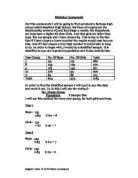
Mode of Girls and Boys Weight
The arithmetic mean of a group of numbers is found by dividing their sum by the number of members in the group; e.g., the sum of the seven numbers 4, 5, 6, 9, 13, 14, and 19 is 70 so their mean is 70 divided by 7, or 10. Less often used is the geometric mean (for two quantities, the square root of their product; for n quantities, the nth root of their product).
Modal Weight Stem and Leaf Diagram
Student IQ Level
Stem
Leaf
Frequency
8
9 9 1
3
9
9 5 6 2 0
5
0
8 0 3 3 0 0 8 0 3 4 0 4 4 1 4 1 2 6 6 3
9
1
6
2
2 4
2
Key 13 / 0 = 130 kg
Average TV hours per week
Stem
Leaf
Frequency
0
2 0 8 6 8 7 6
7
4 6 0 7 4 8 6 0 7 5
0
2
7 2 5 1 1 4 8 8 1 2
0
3
0 6
2
4
0
Histogram
This form of data representation will help me find the spread of data and also the trend in data and the results and firstly below is a histogram showing the IQ levels of my sample:
IQ
Average Hours of TV per week
This shows me the Median Group for IQ Level 100-110 and the Number of Average hours varies Median group of 10-30
Variance and Standard Deviation
Variance is a measure of the spread of the distribution and the square root of the result in the Standard Deviation. This can be calculation using a certain formula, which is shown below. By completing this statistical task it will help me measure the spread of the data and the mean of the distribution.
Standard Deviation Formula:
Below I will now produce a table in which I will calculate the standard deviation for firstly the IQ and then the Average Hours of TV:
IQ Levels
IQ Level (Midpoint of Group)
85
95
05
15
25
Frequency
3
5
9
2
The Mean Is
(3 X 85) + (5 X 95) + (19 X 105) + (1 X 115) + (125 X 2)
= 3090/30= 103
30
And the standard deviation will be
V [2 X (85-103)] + [5 X (95 - 103)] + [19 X (105-103)] + [1 X (115-103)]
+ [2 X (125-103)
30
V 18/30 = 0.7746 4.dp
I will now complete the same Standard Deviation Calculation as I had produced but in this particular case I will do the Deviation and Spread of Data on Average Hours per Week per student
Average Hours Per week TV
Average Hours Per TV week (Midpoint of Group)
5
5
25
35
Frequency
7
0
0
3
The Mean Is
(5 X 7) + (10 X 15) + (10 X 25) + (3 X 35)
= 540/30= 18
30
And the standard deviation will be
V [7 X (5-18)] + [10 X (15 - 18)] + [10 X (25-18)] + [3 X (35-18)]
30
V 1/30 = 0.0333 4.dp
Conclusion
From the Standard Deviation that I have come to find how spread out the data that I have used in my sample for this particular hypothesis and measure of the dispersion of the data and has helped me see whether the data I have is unbiased and of a sufficient spread and size and it will also help me measure the reliability of the sample that I have taken is that it is reliable which is usual on a scale between -1 to 1 and also that the spread of data in the IQ levels in larger than the Average TV hours watched which shows me that in my final evaluation the results for Average TV hours watched per week will be generally more accurate and conclusive.
Standardised Scores
I will now find the Standardised score for 5 students from my sample at Random. It will help me compare the values.
5 Student that I have chosen for this calculation are:
1
Flawn
Elise
Neighbours
0
01
0
Grimshaw
Katie
Blind Date
7
04
1
Cripp
Justin
M.T.V. Base
24
00
Standardised Scores Calculation/Formula
Score - Mean
Standard Deviation
Elise
Katie
Justin
Mean
Standard Deviation
IQ Level
01
04
00
03
0.7746
Average Hours TV Per Week
10
7
24
8
0.0333
Elise Standardised Scores
IQ Level = (101-103) / 0.7746 = - 2.58
Average TV Hours = (10-18)/0.033 = -240
Katie Standardised Scores
IQ Level = (104-103) / 0.7746 = 1.29
Average TV Hours = (17-18)/0.033 = -30.30
Justin Standardised Scores
IQ Level = (100-103) / 0.7746 = - 3.87
Average TV Hours = (24-18)/0.033 = 181
From this I find that that Katie has the better standardized result since her results is a positive figure whereas as Justin's standardized score was a negative value and Elise has the best Average TV house standardized score.
Time Series Line Graph
A Line graph is used to display data when the two variables are not related by an equation and you are not certain what happens from one point to another. I will need to plot this graph extremely carefully due to the fact I cannot enter all the data in my sample and produce this graph since there will no trend which I will be able to view so I will viewing student at different Average Heights in Order and then Plot their IQ Levels on a Line Graph and from this I will able to make a trend comparison. The Line graph will consist of TWO Variables.
On the Whole it is very compact and difficult to give a definite conclusion according to this graph due to the fact the trend is fluctuation up and down and very slightly and upward trend although it is very difficult to tell and verify and form an definite answer to the hypothesis that I have chosen to investigate. Also in addition to this the verification are rather minor and steady and fluctuate largely. Also I can add to this that the basic IQ level is not efficient and excessively effected by the Number of Hours of TV you but generally your age and your understanding and knowledge overall.
Conclusion/Evaluation of Hypothesis 1
In my honest opinion I feel that I successfully completed and analyzed my hypothesis and I have gained a sufficient evidence to back up my theories. I would like to remind you that my main objective for this hypothesis was to find out whether I was correct or incorrect in my thinking that Boys at Mayfield School are taller and weigh more on average than the Girls at the same school. Within this aim I was also aiming to find whether there is a certain trend or relationship between the height and weight of the students that I have chosen to analyze and as I explained earlier due to the large number of students I was not possible to analyze all students so I gained a sufficient sample which I made as unbiased as possible. MY HYPOTHESIS WAS CORRECT
> The Histograms, frequency polygons proved that the results were more accurate and made more sense than that from the random sampling.
> There is a positive correlation between height and weight. In general tall people will weigh more than smaller people.
> In general boys tend to weigh more and be taller then girls.
> By doing stratified sampling, there were a fewer exceptional values caused by different year groups and therefore ages. I was bound to find irregularities within my data
> The cumulative frequency curves confirm that boys have a more spread out range in weight, with more girls having smaller weights. In height, boys tend to be taller.
> The spearman rank correlation coefficient shows that the correlation between height and weight is strong.
> My Body Mass Index showed that there is a strong trend between height and weight
> In general the taller a person is, the more they will weigh.
> There is a positive correlation between height and weight. In general tall people will weigh more than smaller people.
> There therefore is a positive correlation between height and weight across the school as a whole. This correlation seems to be stronger when separate genders are considered
> If I had taken larger samples my hypothesis may become more accurate.
Conclusion/Evaluation of Hypothesis 2
'Students who watch more hours of TV on average have a Lower IQ Level.
I feel that I have successfully completed and investigated my hypothesis to an extent in which I can be sure of my accuracy of my conclusion and I gained many sufficient forms of evidence. As stated above my hypothesis was to find whether Students who spent a large sum of time per week watching TV have a lower IQ Level and I had come to find that my theory was incorrect to a certain level. I had used many statistical representations to prove my theory.
I was also aiming to find whether there was a regular trend between the two variable and aimed to make my hypothesis as unbiased as possible.The Histogram that I had produced showed that my results were unbiased and relatively accurate in comparison the stratified choice of methods and made more sense on the whole.There is a very weak positive correlation between IQ and TV hours although it is not enough to prove whether my theory was correct and there was not a strong positive correlation that I had expected. In general IQ Level does not increase an Hours of TV increase.Some irregularities were found. The Standardised Score and Standard Deviation help me find the spread of the data so the sample is unbiased and insufficient.
If I had taken large sample my hypothesis may become more accurate and able to form a successful conclusion. The IQ also depends on the persons surrounding, ability and knowledge and stimulation and motivation which can all play a factor in the results.Overall I have found that my Hypothesis was incorrect and the statistical evidence that I had gained did not back up my theory. Another reason behind my misfortune is the range of data from 7-11 is too wide and I should have narrowed the frame down but now helps me in the future.
Mathematics Statistics Coursework
- 1 -Elliott Greenman 11DB