Maths Portfolio 1 Logans logo
IBO INTERNAL ASSESMENT
LOGAN'S LOGO
MATHEMATICS SL TYPE II
INTRODUCTION
Logan has designed the logo at the right. The diagram shows a square which is divided into three regions by two curves. The logo is the shaded region between the two curves.
He wishes to find mathematical functions that model these curves.
In order to find these functions, we will need to overlay the logo on graph paper, so we can interpret data points to be able to plot them.
Take note that in the "modeling the data" in the next section, the logo was not resized, but set as transparent so that data points could be read.
Also, take into consideration the uncertainty of the measurements (± 0.25 units). For modeling purposes, the uncertainties are not included in the data calculations; however this should not be overlooked.
MODELING THE DATA
NOTE: Data tables and their graphs are included on the next page.
TOP CURVE :
In order to find a function to model the top curve, there are various methods that we can use. One is to overlay the logo onto a set of axes and estimate points for the function. Once we obtain these points, we can then plot them onto a new set of axes. Judging from the logo itself, at first glance it appears that a sine function would fit the data. The sine function would have to undergo a series of transformations to eventually fit the curve.
Using the axes and logo depicted above, I estimated 13 points for and recorded them in the data table below:
NOTE: Due to the limited precision of the graph, I was only able to estimate to the nearest tenth. Maximum and minimum points have been shaded.
X
Y
-2.5
-1.0
-2.0
-2.5
-1.6
-2.8
-1.0
-2.4
-0.5
-1.3
0.0
0.0
0.5
.5
.0
2.6
.5
3.4
.8
3.5
2.0
3.4
2.5
2.5
2.6
.9
After determining these data points, I then plotted them onto a separate set of axes:
From here, it is obvious that a sine function would fit the data. A sine function can be defined as:
,
Where a represents the amplitude of the sine curve (or vertical dilation); b is the horizontal dilation; c is the horizontal shift; d is the vertical shift; and x and y are the width and length in units respectively.
TO FIND a:
As mentioned above, changing the variable a will affect the amplitude or vertical dilation of the sine curve. This is a dilation of the sine curve parallel to the y-axis, and does not affect the shape of the graph. The amplitude of the function is the distance between the center line (in this case the x-axis) and one of the maximum points. In order to determine the value of variable a, we must first look at the maximum and minimum (highest and lowest) points on the curve, which are (1.8, 3.5) and (-1.6, -2.8) respectively. When we find the amplitude of a sine curve, we can disregard the x-values, as they do not tell us anything about the height of the curve.
Now that we've found the highest and lowest points of the sine curve, we must divide the difference between the two y-values (subtracting the highest point on the y-axis from the lowest will give us the actual height of the curve) by 2:
The value of a, 3.15 units, is the vertical dilation of the curve because it reflects the stretch factor compared to the original sine curve (defined as ), where the amplitude is 1 unit.
However, 3.15 is not the final value of a. It can be seen from the above graph that the curve begins with a negative slope (it goes downwards first and then upwards). This indicates to us that we must place a negative sign before the a value, so the curve will begin with a negative slope. Thus, the final value of a=-3.15.
TO FIND b:
As stated above, changing the variable b will affect the horizontal dilation of the sine curve. This dilation occurs parallel to the x-axis, which means that the period of the graph is altered. A period is defined as the length it takes for the curve to start repeating itself. Thus in order to determine the variable b's value, we first need to look at the period of the graph. For the original sine curve, the period is, or 360º . Thus the formula that relates the value of b to the period ? of the dilated function is given by:
,
Since the graph of will show b cycles in 2? radians. From this equation we see that as the value of b is increased (the horizontal dilation of the curve is greater), the period becomes smaller. We know this because b is the denominator, meaning that increasing its value would decrease the overall fraction's value.
To find ?, it was easier to find half of the period first, and then double it to ensure accuracy. Going back to the definition of a period, how long it takes for the curve to repeat itself, it makes sense then that by finding the difference between the x-values of the maximum and minimum points on the curve, we would find half the period. The maximum value is (1.8, 3.5) and the minimum is (-1.6, -2.8). We can now substitute the x-values of these two points into the period equation to find b:
TO FIND c:
As previously stated, changing the variable c will affect the horizontal shift of the sine curve, so thatare translations to the right, whileare translations to the left. The original sine curve starts (meaning it crosses the center line of its curve) at point (0,0), and using this point as a reference, I can determine how many units leftwards my curve has shifted. (I know it has shifted leftwards after comparing my graph to the original sine graph). Therefore, to find the value of c, I must first determine the center line of my curve ...
This is a preview of the whole essay
TO FIND c:
As previously stated, changing the variable c will affect the horizontal shift of the sine curve, so thatare translations to the right, whileare translations to the left. The original sine curve starts (meaning it crosses the center line of its curve) at point (0,0), and using this point as a reference, I can determine how many units leftwards my curve has shifted. (I know it has shifted leftwards after comparing my graph to the original sine graph). Therefore, to find the value of c, I must first determine the center line of my curve - the middle line of the total height. In fact, we already determined this when we found variable a. (Recall that we divided the total height of the curve by 2 to find the amplitude). The total height of the sine curve is 6.3 units, and divide this by 2 to get 3.15 (variable a).
However, when we graph, it is clear that this line is not the center line of the curve:
From here, we must then add the minimum y-value (-2.8) to obtain a number that we can graph onto the axes. 3.15+-2.8=0.35.
Now, having graphed onto the axes, I can visually determine the horizontal shift of my graph. By extending the data points I plotted to meet the center line of the curve, I was able to estimate how many units leftwards my graph had shifted. This is shown on the graph by the circled red point.
Going back to the original sine curve as a reference:
For the original sine curve, we know the center line is the x-axis, and we see that the original sine curve starts at (0, 0) - represented diagrammatically by the circled red dot. We can now compare my graph to see what the horizontal shift should be. The starting point for the original sine curve is (0, 0) while the starting point for my curve is (-3.0, 0.35). Thus, I determined the value of c=3.0.
TO FIND d:
As previously mentioned, changing the variable d will affect the vertical shift of the sine curve. If d>0 the graph is shifted vertically up; if d<0 then the graph is shifted vertically down. Thus adding or subtracting a constant to the sine function translates the graph parallel to the y-axis. To calculate the value of d here, we make use of the following equation:
,
Which will work because if you add the highest and lowest y-value points of the curve together, then divide by 2, the result would give you an estimate of the position of the x-axis - if it was merely a graph of .
Notice that this value of d is the exact same y-value we calculated when we were determining variable c, by extending the data points of my curve to meet the center line. Thus, d=0.35.
To recap the determined values for each of the variables, we have:
a=-3.15
b=
c=3.0
d=0.35
y=-3.15sin(1.01x+3.0)+0.35
Combining the determined values of a, b, c, and d, we now have a complete sine function to fit the data with:
This then gives us the following graph:
The curve overall is a good fit, However, we can see that in the red circled area, there are points that the curve doesn't fit very well. This means that the horizontal stretch factor, or variable b is a little off, and we need to increase it. Let's try changing it from 0.92 ( rounded to the nearest hundredth) to 1.01.
Comparing the turquoise with the green curves, we can conclude that the turquoise one is a better fit. This gives us a final equation for the top curve to be:
Now we just need to restrict the domain and range to the parameters we set at the beginning of the investigation. The final graph is shown at the left.
The small adjustments we made at the end exhibited the error in our calculations to find the curve of best fit. This can, in turn, be attributed to the large uncertainty in obtaining the actual data. Because I was only able to read points off of the graph, smallest of 1 unit, my precision was limited to one decimal place, and the uncertainty was quite large (±0.5 units). Another limitation was the thickness of the line in the original logo. Because it was so thick, it was also hard to determine where exactly the points lied. This increased the uncertainty of our measurement. Therefore, small adjustments to the curve were needed at the end to ensure the function best matched the data.
BOTTOM CURVE :
In order to find a function to model the bottom curve, we can also take the sinusoidal function approach.
Again, using the axes and logo depicted above, I estimated 13 points for and recorded them in the data table below:
NOTE: Due to the limited precision of the graph, I was only able to estimate to the nearest tenth. Maximum and minimum points have been shaded.
X
Y
-2.5
-3.1
-2.0
-3.5
-1.5
-3.4
-1.0
-2.6
-0.5
-1.8
0.0
-0.8
0.5
0.1
.0
0.7
.4
0.9
.5
0.8
2.0
0.3
2.5
-1.0
2.6
-1.6
After determining these data points, I then plotted them onto a separate set of axes:
From here, it is obvious that a sine function would fit the data. A sine function can be defined as:
,
Where a represents the amplitude of the sine curve (or vertical dilation); b is the horizontal dilation; c is the horizontal shift; d is the vertical shift; and x and y are the width and length in units respectively.
TO FIND a:
As mentioned above, changing the variable a will affect the amplitude or vertical dilation of the sine curve. This is a dilation of the sine curve parallel to the y-axis, and does not affect the shape of the graph. The amplitude of the function is the distance between the center line (in this case the x-axis) and one of the maximum points. In order to determine the value of variable a, we must first look at the maximum and minimum (highest and lowest) points on the curve, which are (1.4, 0.9) and (-2.0, -3.5) respectively. When we find the amplitude of a sine curve, we can disregard the x-values, as they do not tell us anything about the height of the curve.
Now that we've found the highest and lowest points of the sine curve, we must divide the difference between the two y-values (subtracting the highest point on the y-axis from the lowest will give us the actual height of the curve) by 2:
The value of a, 2.2 units, is the vertical dilation of the curve because it reflects the stretch factor compared to the original sine curve (defined as ), where the amplitude is 1 unit.
However, 2.2 is not the final value of a. It can be seen from the above graph that the curve begins with a negative slope (it goes downwards first and then upwards). This indicates to us that we must place a negative sign before the a value, so the curve will begin with a negative slope. Thus, the final value of a=-2.2.
TO FIND b:
As stated above, changing the variable b will affect the horizontal dilation of the sine curve. This dilation occurs parallel to the x-axis, which means that the period of the graph is altered. A period is defined as the length it takes for the curve to start repeating itself. Thus in order to determine the variable b's value, we first need to look at the period of the graph. For the original sine curve, the period is, or 360º . Thus the formula that relates the value of b to the period ? of the dilated function is given by:
,
Since the graph of will show b cycles in 2? radians. From this equation we see that as the value of b is increased (the horizontal dilation of the curve is greater), the period becomes smaller. We know this because b is the denominator, meaning that increasing its value would decrease the overall fraction's value.
To find ?, it was easier to find half of the period first, and then double it to ensure accuracy. Going back to the definition of a period, how long it takes for the curve to repeat itself, it makes sense then that by finding the difference between the x-values of the maximum and minimum points on the curve, we would find half the period. The maximum value is (1.4, 0.9) and the minimum is(-2.0, -3.5). We can now substitute the x-values of these two points into the period equation to find b:
TO FIND c:
As previously stated, changing the variable c will affect the horizontal shift of the sine curve, so thatare translations to the right, whileare translations to the left. The original sine curve starts (meaning it crosses the center line of its curve) at point (0,0), and using this point as a reference, I can determine how many units leftwards my curve has shifted. (I know it has shifted leftwards after comparing my graph to the original sine graph). Therefore, to find the value of c, I must first determine the center line of my curve - the middle line of the total height. In fact, we already determined this when we found variable a. (Recall that we divided the total height of the curve by 2 to find the amplitude). The total height of the sine curve is 4.4 units, and divide this by 2 to get 2.2 (variable a).
However, when we graph, it is clear that this line is not the center line of the curve:
From here, we must then add the minimum y-value (-3.5) to obtain a number that we can graph onto the axes. 2.2+-3.5=-1.3.
Now, having graphed onto the axes, I can visually determine the horizontal shift of my graph. By extending the data points I plotted to meet the center line of the curve, I was able to estimate how many units leftwards my graph had shifted. This is shown on the graph by the circled blue point.
Going back to the original sine curve as a reference:
For the original sine curve, we know the center line is the x-axis, and we see that the original sine curve starts at (0, 0) - represented diagrammatically by the circled red dot. We can now compare my graph to see what the horizontal shift should be. The starting point for the original sine curve is (0, 0) while the starting point for my curve is (-3.4, -1.3). Thus, I determined the value of c=3.4.
TO FIND d:
As previously mentioned, changing the variable d will affect the vertical shift of the sine curve. If d>0 the graph is shifted vertically up; if d<0 then the graph is shifted vertically down. Thus adding or subtracting a constant to the sine function translates the graph parallel to the y-axis. To calculate the value of d here, we make use of the following equation:
,
Which will work because if you add the highest and lowest y-value points of the curve together, then divide by 2, the result would give you an estimate of the position of the x-axis - if it was merely a graph of .
Going back to the equation:
Notice that this value of d is the exact same y-value we calculated when we were determining variable c, by extending the data points of my curve to meet the center line. Thus, d=-1.3.
To recap the determined values for each of the variables, we have:
a=-2.2
b=
c=3.4
d=-1.3
y=-3.15sin(1.01x+3.0)+0.35
Combining the determined values of a, b, c, and d, we now have a complete sine function to fit the data with:
This then gives us the following graph:
However, we can see, in the blue circled area, places where the curve doesn't fit the data well. This means that the horizontal stretch factor, or variable b is a little off, and we need to increase it. Let's try changing it from 0.92 ( rounded to the nearest hundredth) to 1.01.
Comparing the turquoise with the green curves, we can conclude that the turquoise one is a better fit. This gives us a final equation for the bottom curve to be:
Now we just need to restrict the domain to the parameters we set at the beginning of
the investigation.
The final graph is shown at the left.
The small adjustments we made at the end exhibited the error in our calculations to find the curve of best fit. This can, in turn, be attributed to the large uncertainty in obtaining the actual data. Because I was only able to read points off of the graph, smallest of 1 unit, my precision was limited to one decimal place, and the uncertainty was quite large (±0.5 units). Also, another limitation was the thickness of the line, which prevented me from reading the data clearly.
ADJUSTING THE DATA
Logan wishes to print t-shirts with the logo on the back. She must double the dimensions of the logo for this purpose. Thus, the functions I just developed must be modified if the dimensions are changed.
If the dimensions of the logo are doubled, then both of the curves' width and length must be increased by a factor of 2. In order to do this, variables a, c and d must be multiplied by 2, while variable b must be divided by 2.
Variable a: The amplitude would have to be multiplied because, as it is responsible for the vertical dilation of the curve, it stretches the graph vertically. Multiplying this by 2 would result in all the y-values being multiplied by 2, thus vertically stretching the graph by a factor of 2.
Variable b: The horizontal dilation factor would have to be divided by 2. Remember that this variable is indirectly linked to the period of the curve. If the dimensions are doubled, then the period must also be doubled; however, doubling the period has the reverse effect on the actual variable b. If the original period was ? for example, and was doubled to 2? - what would happen to b?
?=?
?=
?=
b=2
?=2?
?=
2?=
b=1
We can see that by doubling the period, we have to divide the variable b by 2.
Variable c: The horizontal shift would have to be multiplied by 2. Again, doubling the dimensions will double the size of the logo, and in order to compensate for this, the horizontal shift has to be doubled as well.
Variable d: The vertical shift would also have to be multiplied by 2 for the same reason as variable c. The new logo on the t-shirt will be doubled from the original, meaning that the width would be doubled. Naturally, the vertical shift has to be multiplied by 2 to compensate for the change.
Finally, the parameters would have to be doubled. The original logo's parameters were:
The new t-shirt logo's parameters will be:
and represent the top and bottom curves respectively before resized to put on the t-shirt (shown by the pink and blue lines, respectively). and are the new curves, resized to print on the t-shirt (shown by the green and black curves, respectively.)
Logan also wishes to print business cards. A standard business card is 9cm by 5cm. In order to print the logo onto the business cards, the functions I have developed must be modified so that the logo extends from one end of the card to the other. Firstly, the domain and range must be adjusted.
At the present, the dimensions for the logo are 10cm × 9.4cm and the parameters are:
Because the logo is on a set of axes that is measured in units and not centimeters, we need to be able to convert between the two. From the domain above, we find that the length of the logo on the graph is 5.2 units, which is proportional to 10cm. From the range, we calculate the width of the logo on the graph to be 8 units, which is proportional to 9.4cm.
So we have for the domain and for the range.
Logan wishes to reprint the logo onto business cards, dimensions of 9.0cm × 5.0cm. Using the above conversion factors, we find the parameters to be: and
Sample Calculation:
Thus, to make the appropriate changes, the present parameters for the domain must be multiplied by in order to shrink the domain from 10cm to 9cm. The fraction was obtained by setting the numerator equal to the desired domain and the denominator equal to the original domain. However, we have already established that there are 2 different sets of measurement and cannot use the 2 interchangeably. Thus we must convert the multiplier to units. We do this by following the same methodology as we did for cm, and find that the domain must be multiplied by to shrink the logo from 10cm to 9cm:
Present Domain=
Domain minimum= -2.5units × =-2.55units
Domain maximum= 2.7units × =2.43units
New Domain=
We need to make the same changes to the original range. This time, we need to multiply the existing minimum and maximum limitations for the range by (again putting the desired range over the original range) to achieve the same effect. And again, we must change this conversion factor from cm to units, and find that the range must be multiplied by to shrink the logo from 9.4cm to 5cm:
Present Range=
Range minimum= -4.0units × =-2.1275units
Range maximum= 4.0units × = 2.1275units
New Range=
We now must adjust the function itself, having already manipulated the parameters for it. To do so, we must distinguish which variables will be altered given the new domain and range.
There are 4 variables in the general sine function:
Which directly correspond to the 4 features that define a sine curve:
. Amplitude (vertical dilation) - a
2. Period (b is the horizontal dilation) - b
3. Horizontal shift- c
4. Vertical shift- d
Numbers 1 and 4 both stretch or shrink the curve parallel to the x-axis, which means that the amplitude a and vertical shift d will only be affected by the manipulated range (factor of or). On the other hand, numbers 2 and 3, the horizontal dilation and shift, will stretch or shrink the curve parallel to the y-axis. Again, this means that they will only be affected by the manipulated domain (factor ofor).
Now we are able to apply the corresponding shrink factors to their appropriate variables in order to obtain a new curve for Logan's business cards.
TOP CURVE
The final equation for the top curve is given by the following equation:
with a period of 6.3.
Thus we must make the following changes to each of the variables. For a, the amplitude or vertical dilation factor:
For b, the horizontal dilation factor:
For c, the horizontal shift factor:
For d, the vertical shift factor:
Thus the final equation for the logo with dimensions compatible with that of a standard business card is: with parameters of: and.
The graph of the manipulated curve is shown below, on a 9cm × 5cm business card.
BOTTOM CURVE
The final equation for the top curve is given by the following equation:
with a period of 6.0.
Thus we must make the following changes to each of the variables. For a, the amplitude or vertical dilation factor:
For b, the horizontal dilation factor:
For c, the horizontal shift factor:
For d, the vertical shift factor:
Thus the final equation for the logo with dimensions compatible with that of a standard business card is: with parameters of: and.
The graph of the manipulated curve is shown on the next page, on a 9cm × 5cm business card.
The final logo on the business card is shown below. Note that the dimensions are in units which, shown through the calculations above, have been converted to ensure they match the ratio and proportion of a standard business card.
33 | Page
Natalie Sullivan 13SAW Maths SL