For business area, this model commonly used to analysis pure competition, which assumes may buyers and sellers in the market. Linear programming can let the manger make decision to choose the opportunities facing an organization regarding the optimum use of its long-term resources to change from one time period to another. To make the best decision, it is important choose the best profit to run the organization.
Chapter 2 Applications - Case study
Case study
A clothing manufacturer makes football jerseys and soccer shirts for youth teams. The major resources used are material, numerals, and labour. Football jerseys required 8 square feet of material, soccer shirts 5 square feet. Both jerseys and shirts require two numerals. It takes two hours to make a football jersey and three hours to make a soccer shirt. The company currently has 215 square yards of material,600numberals,and685 hours of labour available .Each football jersey yields a profit of $6 and each soccer shirts $4.50.Formulate the Linear Programming model for the correct production mix.2
Solution
Consider the manufacturer case study above .the constraints were:
F=number of football jerseys
S=number of soccer shirts
F≥0;
S≥0;
8F+5S≤1935;(Because one yard makes three feet. So, one square yard makes nine feet)
2F+2S≤600;
2F+3S≤685;
The objective function was: the contribution to profit from each price:
Max: 6F+4.5S
Solve this problem graphically.
Step 1: choose the axes
Firstly, the variable axis needed to be decided. Here either is suitable .The writer Choose to plot F on the x-axis and S on the y-axis.
Step2: Plot the constraints
Turning all the constraints into equalities it need to plot three lines:
Line one :8F+5S≤1935 (material)
Line two:2F+2S≤600(numerals)
Line three:2F+3S≤685(hours)
Line one: Assume 8F+5S=1935. When F=0, it will have 5S=1935. Then, S=387.Similarly when S=0,it will have 8F=1935,then F=241.875≈242.
Line Two: Assume 2F+2S=600. When F=0, it will have 2S=600. Then, S=300.Similarly when S=0,it will have 2F=600,then F=300.
Line Three: Assume 2F+3S=685. When F=0, it will have 3S=685. Then, S=228.Similarly when S=0,it will have 2F=685,then F=343.
The three lines are plotted in the figure 1.1
Each side of the line required to the left as all our inequalities are ≤.The region satisfied by all the constraints is the feasible region: any point lying in this region is a possible solution to the problem of optimising the contribution to profit.
Figure 1.1
Step 3: Choose arbitrary values.
Combine any two of the functions .The writer choose the functions of Line one :8F+5S≤1935 (material) and line two:2F+3S≤685(hours) to solution it .
Assume 8F+5S=1935 and 2F+3S=685.
8F+5S=1935 (1)
2F+3S=685 (2)
Let (2)*4 change to :8F+12S=2740. Then use (2)minus(1).Let 7S=805,S=115.
And then ,let S=115 put in (2),then 2F+3*115=685 ,F=170.
So, the arbitrary values are F=170, S=115.
Step 4: Find the profit line and extreme points of the feasible region.
Let F=170and S=115 used in the objective function 6F+4.5S. Then, let the objective function equal to 6*170+4.5*115=1537.5≈1538.
To find the feasible region .Let the objective function 6F+4.5S=1538. When F=0, let 4.5S=1538,then S=341.7≈342. Similarly, when S=0,let 6F=1538,then F=256.3≈257.
Next, the writer choose the two function of material and numerals above .so, next according to the point of intersection of this two lines to current position until touch the very edge .To find out the feasible region, the maximize profit.
This Assume profit line will show on figure 1.2
Figure 1.2
Step 5: The best solution.
It can see that the maximum contribution to profit would occur when produce 170
football jerseys with $6 and 115 soccer shirts with $4.5 .
6*170+4.5*115=1537.5
The manufacturer best profit would be $1537.5.
The figure 1.3 feasible regions are the maximum profit.
Figure 1.3
Chapter 3 Analysis and evaluation
The analysis will be in accordance with the case study and changes of any variable of the functions. The changes in the clothing manufacturers of the constraints are considered. Changes in either the labor’s work time or material resources will bring about changes of the profit.
Analysis 1
Originally, there is labor constraint shown as 2F+3S≤685. Now, assume that an increase in labour by five hours a day. The function becomes 2F+3S≤690.
Keep other two constrains unchanged. To solve the functions similar methods are used as above. The other two functions can be solved in the same way. Solve the new function of 2F+3S≤690. Assume that 2F+3S=690.When F=0,S=230,also when S=0,F=345.
Combine two of the functions to confirm the best profit after change the work time.
2F+2S=600 (1)
2F+3S=690 (2)
Solve above equations by subtracting (2) by (1) . The results are S=90 and F=210.
We substitute the values of S= 90 and F= 210 into the objective function of 6F+4.5S=
$1665.Compare with The optimal maximum profit was originally found to be $1537.5. The new calculated result gives an increase in profit of $128 by prolonging five hours a day .It is means that one hour’s additional work can increase profit of $25.6.
From the calculated and related the case study, the following analyses can be given. If the labour’s work time increases one hour, then the profit will increase $25.6.It means that if the labour’s salary exceed $25.6 per hour, then manufactory will not get any profit. Actually, the salary of a manufactory worker is nearly between $8and$9 per hour, it never exceeds $25.6. The result is that no matter the manufactory increase labour’s work time or not, it will get profit.
Analysis 2
Originally, there has material constraint as 8F+5S≤1935. Now, assume that an increase one square yard (nine feet). The function is 8F+5S≤1944.
Keep other two constraints unchanged. To solve the functions use the ways as shown above. Other two function’s solve is the same .solve the new function of 8F+5S≤1944.Assume 8F+5S=1944.When F=0,S=388.8≈389,also when S=0,F=243.
Combine two of the functions to confirm the best profit after change the material.
8F+5S=1944 (1)
2F+2S=600 (2)
Solving it, and subtract it .S=152 and F=148.
We substitute the values of S= 152and F= 148 into the objective function of 6F+4.5S=
$1672.Compare with the optimal maximise profit was originally found to be $1537.5. Which gives an increase in profit of $34.5 by one square yard. It is means that if the price of one square yard material is more then $34.5 the manufacture will not get profit . On the contrary, if the price of one square yard material is less then $34.5 ,the manufacture will get profit .
Chapter 4 Conclusion
The theory and implementation of linear programming are fairly simple. The data to be used for the solution are usually easy to obtain. By means of solving the function and combine the plot can be easy to find the results. Using linear programming to analysis can be applied into many areas. Especially in business area it can be used to do the business planning and control. And in conjunction with the case study, it can be seen that this method is also useful in developing manufacture plans as producing the jerseys and shirts for the youth teams.
In conclusion, these scientific approaches to solving problems are easy way to find out the best profits for a manufacture. Linear programming is the most useful method in making decision no matter the variable will be changed or not. This model can consider those problems that require the most creative attention. Linear programming is a useful model suggesting that management must continually evaluation its original investment decision.
No matter how the variables are changed under certain conditions, the linear programme is aiming at finding out the best way to achieve profits as far as possible in order to run the organization with optimum profits.
REFERENCE
-
Terry I. Dennis and Laurie B.Dennis (1991) management Science New York: West publishing company
BIBILOGRAPHY
-
R. D. Seale&A. D. Sealejr& Jason Leng(2004) An application of business activity modeling to regional production and national distribution of plywood. Forest Products Journal VOL. 54, No. 12
-
Anderson,D.R.,D.J.Sweeney ,and T.A. Williams.(1974) Linear programming for decision making .St.Paual:West publishing
-
Burke,R.,(1995)Project Management-planning &control ,wiley ,London
http://www.markschulze.net/LinearProgramming
Terry l.Dennis and Laurie B.Dennis (1991) management Science New York: West publishing company
2 Terry l.Dennis and Laurie B.Dennis (1991) management Science New York: West publishing company