A business requires reasonable amount of inventory to ensure smooth operation. The inventory problem determines the inventory levels that balances the two extremes ( too much and too little ).The factors that apply in solving the inventory is the demand for an item may be deterministic ( identified with certainty) or probabilistic ( portrayed by a probability solution).
General Inventory Model
The cycle for inventory model is placing and receiving order. This working activity is applied with the inquiries
- How much to order?
- When to order?
The above questions are answered by minimizing the following cost model.
Total Inventory Cost = (Purchasing Cost) + (Setup Cost) + (Holding Cost) + (Shortage Cost).
An inventory system can be based on periodic review or continuous review where new are orders are placed when the inventory level drops to a certain level called the reorder point. There are 2 types of deterministic inventory model static and dynamic. The static model has constant demand over time and in the dynamic model the demand changes over time.
Deterministic Inventory Model
Static Economic Order Quantity
The simplest inventory model involves constant rate demand with instantaneous order replenishment and no shortage define by
Y = √2KD/h unit every t0 where,
Y = Ordered Quantity
D = Demand Rate
K = Setup Cost
h = Holding Cost
t0 = Ordering Cycle
The above equation reflects the instantaneous arrival of order on placement .Instead a positive lead time L may occur between the placement and receipt of an order. In this case a reorder point occurs when the inventory level drops to LD units. Now effective lead time becomes
Le = L- nt0
Where n is the largest integer no exceeding L/ t0.The following figure provides the pictorial representation of the static EOQ method.
The realistic inventory model. Q = order batch size, B = order point, S = the buffer inventory, L = order lead-time.
Dynamic EOQ Model
This model differs from the static model in 2 aspects
- The inventory level is reviewed periodically over finite number of equal periods
- The demand per period is dynamic in the sense that it may vary from one period to the next.
The situation in which dynamic deterministic demand occurs is material requirement planning MRP
Probabilistic Inventory Model
The technique presented in the above method assumes that data area known with certainty which is not true for all situations and there are several cases in which it is not correct to represent the demand by a single deterministic value. In such cases we observe the historical data to represent the demand as a probabilistic distribution
Probability is associated with performing an experiment whose outcome occurs randomly. The conjunction of all the outcomes of an experiment is referred to as the sample space and subset of the sample space is known as an event.
The developed probabilistic model is broadly categorized under continuous and (Single & Multi) periodic review situations.
Continuous Review Model
There are 2 approaches in this model
- Probabilitized EOQ Model
- An EOQ Model with probabilistic demand in the formulation.
Probabilitized EOQ Model
This is an improvised version of deterministic EOQ Model to reflect the probabilistic nature of demand by using an approximation that superimposes a constant buffer stock on the inventory level throughout the entire planning horizon .The size of the buffer is determined such that the probability of running out of stock during lead time does not exceed the pre specified value.
It is given by,
P {XL ≥ B + µL} ≤ α
Where
L = Lead Time
XL = Random variable representing demand during lead time.
µL = Average demand during lead time.
B = Buffer stock value.
α = Max allowable probability of running out of stock during lead time.
The main assumption in this model is XL the demand during lead time L it is normally distributed with the mean and standard deviation during lead time (σL)
Probabilistic EOQ Model
There are 2 reasons to believe that this model presents the optimal inventory policy. The fact that pertinent information regarding the probabilistic nature of demand is initially ignored only to be revived in a totally independent manner at a later stage of calculation is sufficient to refute optimality. The model calls for ordering the quantity Y when ever the drops to level R as in deterministic case where the reorder R is the function of the lead time .The optimal value of Y and R is determined by minimizing the expected cost per unit time that includes the sum of the setup ,holding and shortage costs.
The model has three assumptions
- Unfilled demand during lead time is backlogged
- No more than one outstanding order is allowed
- The distribution of demand during lead time remains stationary with time.
To develop the total cost function per unit time let
f(x) = pdf of demand x during lead time
D = Expected demand per unit time
h = Holding cost per inventory per unit time
p = Shortage Cost per inventory unit
K = Setup Cost
Based on these definitions the elements of the cost function are now determined
- Setup cost = KD/Y
- Holding Cost = hI where I is the average inventory which is given by
I = (Y+E{R-x})+E{R-x}/2
=> Y/2 + R – E{x}
3. Expected Shortage Cost
When x > R and S = ∫∞R (x-R)f(x)dx
Single- and Multi- Period Models
The classification applies to the probabilistic demand case. In a single-period model, the items unsold at the end of the period are not carried over to the next period. The unsold items, however, may have some salvage values. In a multi-period model; all the items unsold at the end of one period are available in the next period. In the single-period model and in some of the multi-period models, there remains only one question to answer: how much to order.
Trade-offs in Single-Period Models
- Loss resulting from the items unsold
- ML= Purchase price - Salvage value
- Profit resulting from the items sold
- MP= Selling price - Purchase price
- Given costs of overestimating / underestimating demand and the probabilities of various demand sizes.
- How many units will be ordered?
References
- Operations Research: A practical introduction, CRC Press, Boca Raton, London.
-
Operation Research: An Introduction By Hamady .A .Taha (7th Edition).