The storage for point production commodities however displays a different story; this is because there is a very obvious need for storage. By looking at the example of wheat for example if it is harvested at period 1 it is incorrect to assume that all of the wheat produced at period one, will be consumed in period one. The harvest will have to satisfy the demand wheat (which is at this point can be assumed to be constant in all four periods) for each of the four periods and therefore will have to be stored. For point production commodities such as wheat the effect of storage on the product will be minimal because of the nature of the commodity. Therefore even from this simple analysis it can be seen that the marginal benefit from storing commodities which are produced all year round are significantly less than the latter.
I will now focus on the price behaviour of a point production product such as wheat, and explain why such behaviour occurs. I can begin restating my findings from the above discussion that point production commodities are stored throughout the year, and it is the storage of the product which makes it different form commodities which are produced throughout the year. To begin the discussion it is important to note that although the although the product a time t is identical to the product in time t+1, they are treated as two separate economic goods, and the good at t+1 in a economic perspective is like the transformation of wheat into bread, therefore by looking at it from this perspective one would assume economic agents would undertake such an activity if it is profitable to do so (Young).
From the perspective of someone who will be storing the commodity, they will be expecting the price to rise, so the individual or business will store only if they expect a change in price (Et[P1+t] – Pt, Et is the expectations operator). Therefore if the individual or business expect the change in price form period t to t+1 to be negative they would not store the product, or if they found that the price in t+1 would be less than the costs the individual or business has incurred for storage, then they would not store the product.
I will now focus on the costs of storage. First the costs can be physical costs, such as rental of storage costs, handling charges, interest charges etc, and such costs are relatively easy to quantify and so need no further discussion. Another cost could be the marginal risk factor. This is the risk the individual or business has incurred due to storing the commodity because they cannot be certain that their expected change in price will materialise. However the economic agent storing the commodity may be able to reduce their risk, they could do this by storing small amounts, therefore any price deviation from their expected price will result in small, this idea is take from the expected utility framework, which states economic agents will have their welfare reduced as asset holdings become more specialised (Young). However many individuals or businesses will be more inclined to store more commodities therefore maximising their returns from their expectations. Therefore a risk premium should be paid to the holder of stocks to induce them into storing and entering into this risky activity, and that the premium should reflect the volume of the stock held, therefore allowing traders to make the judgement that expected benefits will exceed marginal physical costs.
Another cost the holder of stocks could face is the convenience yield. Sometimes traders may hold stocks to meet the orders of regular customers (Young), in the same way processors (eg millers) may also keep stocks. Millers may keep stocks to take advantage of any price increases however even if the price does not increase, they will still benefit, because for example if there was a problem in the transport system, the extra stocks would come in useful. Therefore it can be said in such a situation that the convenience of having such a stock can give an increase in marginal benefit. The convenience yield is the amount of storage a business has, for example if a miller holds stocks equivalent to six months production, it is unlikely that they would benefit as much, by storing an additional ton (Young).
By summing the three costs above, the following net marginal cost of storage can be derived:
Now I will turn my attention to demand for storage, as this will allow me to analyse the interaction between the supply and demand for storage in a particular period. At this point it is important to keep the demand for storage and the demand for the commodity separate, because they both represent two markets although they are linked. I will be looking at the demand for storage.
The price of the commodity in period t, be equal to Pt = f1 [Ct], where C (consumption) is equal to Ct = St-1 + Xt – St. X is the level of production during the period, and because we are looking at the price behaviour of a point production commodity X will take the value of 1 in one period and will be zero in all other periods. From the consumption formula it can be seen that a change in consumption has effects in the level of stocks. Consider for example if consumption for a period is large, this must mean a reduction of stocks at the end of the period, this will also effect the next period because the opening stocks for the next period will be lower.
Therefore if consumers which to consume more wheat in period t+1, they will require higher levels of stocks to be held at time t (young). The level of demand for storage therefore depends on the expectation of price in the next period, and the price for this period. Consider for example if there is a increase in the expectations operator, this will lead to a fall in consumption in period t+1, and therefore al fall in stocks needed for that period, a increase in price on the other hand will lead to a increase in consumption in period t, therefore a reduction in the amount of stock available at the start of period t+1. There is a negative relationship therefore between the change in price and levels of stock in period t (Young). Therefore the point of intersection of the supply and demand curves determines the level of stocks held at the end of the period and the expected change I the price of the commodity (Young). To create the demand curve for the next period we use the same principles and use the closing stocks as the opening stocks for the next period. The supply curve does not vary over time but the demand curves are different for each period, and each are a function of the other equilibrium stock levels.
However what would happened if a shock was to occur, then expected price will not follow the price trajectory. In this case the model can be adjusted as new information becomes realised. By altering expectations therefore a new trajectory can be formed.
References
Trevor young – course unit guides