A bar chart of marital status makes it visibly obvious that married is the most frequent response. The frequency table shows that 2826 are married 51.4 percent and 51.4 valid percent with no missing cases. The cum percent means nothing with this variable. But what does this tell us about the rest? Living as a couple (co-habitating) widowed, divorced, separated – some have been married.
A better interpretation may be to say that 51.4 percent (just over half) are currently married and 48.5 percent are currently not married. there are 4 (.1 percent) missing cases giving the code value 0.
Highest educational qualifications (AQFEDHI)
Sometimes the order of numbers attached to a variable is significant.
If the possible responses can be arranged in order as with highest educational qualifications, the variable is called ordinal, its codes have an order.
The codes assigned to (AQFEDHI) have an order from high to low.
Highest Degree code 1 First Degree code 2 Teaching Degree code 3 down to No Qualifications code 12.
The cum percentage has some importance with this variable. For example: - the table shows that 20.9 percent have the equivalent or above a higher education qualification or 23.5 percent have above A level educational qualification.
When looking at the bar chart the first impression it gives is that the majority have no qualifications. However, by examining the frequency table and in particular the cum percent column which gives a wider picture. You can see by looking down this column that 63.4 percent have some qualifications and 36.6 percent have none.
There are 20 (.4 percent) miss cases that are given the coding value – 9.
Sex (ASEX)
This is a nominal variable.
Numerical code assigned means nothing
The frequency table shows that: -
There are 2397 males – 43.6 percent – value 1
3104 females – 56.4 percent – value 2
Total 5501 100 percent no missing cases.
The hypothesis I propose is that the political party that a person supports is influenced by their present occupation.
Results of crosstabs procedures:
The dependent variable – Political party supported (AVOTE) are placed in rows.
The independent variable – Register general social class category (the variable doing the influencing) is placed in columns.
(AVOTE) is a nominal variable – the numerical codes assigned mean nothing.
(AJBRGSC) is an ordinal variable – the numerical codes assigned are from highest (professional occupation) code 1 – to (unskilled occupation) code 6.
By just looking at the frequency numbers in the cells the results appear at first surprising. Only 73 of those with professional occupations vote Conservative. The fact that 227 with managerial and technical occupations and only 63 of those unskilled vote Labour was not what I would have imagined. However, when you look at the total number of each column the numbers are very much higher for managerial and technical as they are for skilled non – manual, skilled manual, partly skilled - than they are for unskilled and professional, but this still does not tell you a lot.
What you have to do is look at the percentages in each cell which gives a figure were by each sample adds up to 100. The numbers then turn themselves around, 43.3 percent of those with professional occupations vote Conservative. 44.3 percent of those with unskilled occupations vote Labour against 26.7 percent of those with managerial and technical occupations.
If we stay with those who voted conservative and labour you can see that for those who vote conservative the percentages in the cells get lower has you move across the column from professional occupation to unskilled occupation.
For those who vote labour the percentages in the cells get higher as you move across the column.
This is what I would have expected.
The test shows a high significance of .00000*1
Number of missing observations = 2617
By looking at the frequency table for (AJBSTAT) current labour force status you can see who these missing cases are - unemployed 273, retired 1236, family care159 FT student 159, and so on.
Further Test
Another variable could be added i.e. sex or class together with present
occupations to discover other influences.
BIBLIOGRAPHY
Norusis, M. (1991) The SPSS Guide to Data Analysis for SPSS/Pc+ Chicago: SPSS Inc.