Based on the exposition Of Cullis & Jones we can express a simple algebraic equation of tax incidence in a perfectly competitive industry. In this case we assume a specific tax. For simplicity, partial equilibrium will be used. This is a tax that is expressed as an amount per unit of good. This tax is the difference between what the consumer paid and what it received by the supplier. The former being represented by Pd and the latter by Ps.
This relationship would look like this.
Pd – Ps = t
If we take changes in the tax the equation becomes the following:
dPd – d Ps = dt
Where the “d” stands for differential. At this point to find out how much quantities change when the price changes we simply use the slope of demand or supply curve:
dQd = Dp * dPd
Dp (<0) is the slope of the demand curve. If we multiply the change in Pd ( which is the price paid by consumer) by the slope this gives the corresponding change in quantity demanded. By the same logic the supply curve holds to get
DQs = Sp * dPs
We will now use dPd – d Ps = dt to substitute dPs out of the previous equation.
dQs = Sp *( dPd - dt )= Sp * dPd –Sp * dt .
This is done so that supply is equal to demand after the tax is introduced it must be the case that the change in quantity demanded has to be equal to the change in quantity supplied so:
dQs = dQd
Hence rewriting the previous equation we get
Dp *dPd = Sp * dPd –Sp * dt .
Rearranging everything we get
Sp * dt =(Sp - Dp )dPd
dPd
dt
= Sp .
Sp – dp .
This is an expression for the incidence of tax on the consumer price and is a positive number. We get a more intuitive expression by multiplying above and below by the ratio of price to quantity.
dPd
dt
= Sp (P/Q).
Sp (P/Q) - Dp(P/Q)
If we consider es to be the elasticity of supply and ed to be the elasticity of demand we get the following equation
es
es – ed
The expression ranges from 1 to 0 .Similarly we can get a similar equation for supply. If we continue explaining the example of the specific tax we can say the following. A sales tax of 50 cents per unit with an elasticity of demand of –4 and an elasticity of supply of 0.6, the price paid by the consumer rises by 30 cents or 60 %. { 0.6/(0.6-(-0.4)} = 0.6.
This last equation brings us to a very important concept. In fact the determinants of a tax being shifted are mainly elasticity of demand and supply for both inputs and outputs. In order to explain this concept one can adopt the following example. Let us consider the supply and demand for a good as shown in the figure below.
In this diagram the initial equilibrium before the tax is at E1, with 10 untits sold at the price of Lm 3. At this point the state intervenes introducing a sales tax of Lm 1 per unit. This sales tax will be collected by the sellers. According to the elasticities of demand and supply we can see who will bear cost of this introduction of sales tax by the government.
Since this is a sales tax the initial effect of this tax is to shift the supply curve to the left from S1 to S2. This shift is equivalent to the full amount of the sales tax(i.e. Lm 1). If we consider quantity supplied 13 units ( point A), we can see that before the tax was introduced would ask for Lm 4 per unit in order to sell this given quantity. After this tax is introduced we see that sellers are no longer willing to accept Lm 4 to supply 13 units. Now that the sales tax is introduced they would ask for LM 5(point B). This is done so that the sellers would not be influenced by the tax that they are now required by law, to give to the state. Any point on S2 will be LM 1 greater than the equivalent point on S1.
We can see from the diagram that the equilibrium has moved from E1 to E2. Price moves upwards from Lm 3 to Lm 3.20. In this case buyers burden is limited to 20 cents of the burden while sellers would have to pay the remaining 80 cents left imposed by the state. We should not forget that the entire Lm 1 goes to the state. This means that the seller would receive LM 2.20.
It is clear that in the diagram buyers bear a lighter share of the burden. This takes place because of the responsiveness of consumers to changes in prices. In economics we refer to this phenomenon as elasticity, In fact in this case we can say that demand is more elastic than supply. This could mean that the good we took into consideration is not a necessity good and therefore not inelastic. A small change in price will affect the demand of the consumers. This will hinder producer to pass or shift the burden of the sales tax to the public.
If we look at the following diagram the opposite takes place.
As we see here the supply is more elastic than demand. Hence, this means that the sellers are more responsive to changes in price. In this case the sellers bear a lighter burden than before. This diagram once more reproduces the demand and supply of people for a particular good. As we see from the diagram the equilibrium moves from E1 to E2. In this case as the arrows show that the consumer bear the 80 cents increase in tax whilst the producer just the 20 cents. In this case the seller is able to push almost the full amount of the tax to the consumers.
In order to understand this concept better it is important not to leave the theory in a vacuum, it is important to specify the contexts of which it is used. Therefore one can apply the theory of tax shifting and tax incidence and its determinants to particular scenarios. The analysis used till now was based on the assumptions of perfect markets. However in reality markets are not always perfect. That is why we have to take into considerations some imperfections. If we consider a specific (unit tax) under a condition of a monopoly we can see if things change. The following figure will illustrate this.
AR and MR represent respectively average revenue and marginal revenue before tax, whilst MC represents marginal cost. Equilibrium is found at the point where MC + MR (profit maximization point), with an output of OA, while price equal OB. If we assume that a specific tax of u is imposed, the immediate effect is to shift the MC to MC’. This will bring output to shrink to OC and price rise to BD. The unit tax magnitude is shown by EH. As regards to tax revenue this would amount to area EHGF. Similarly to the perfectly competitive case, changes in output, price and revenue depend on the elasticities of demand and supply.
Now we can observe the effects of a tax on wage income in the same environment of imperfect competition. In reality wages are not determined in a perfectly competitive environment. In fact other than productivity are responsible for the setting of wages. A large proportion of the wages are set in Collective bargaining agreements. These collective bargaining agreements also affect the nonunionized sector. What is interesting to see is if unions are able to enter any increase in taxes on wages in the collective agreement. This does not happen if unions and employers have already agreed on the best bargain, which the unions were able to obtain. Moreover governments must know the economic implications of the incidence of tax, since this can affect economic growth and stability. Heavy rates on wages reduce savings. Since investments depend on savings, the former will also be reduced. A rate structure that hits lower incomes reduces current consumption and correspondingly encourages growth by permitting larger savings.
If we consider perfect markets as regards payroll tax, we know that it is indifferent whether the tax is imposed on the buyer or the seller. Payroll taxes are used largely to finance pension schemes and unemployment benefits. It is therefore indifferent since most payroll taxes fall in two equal parts, half levied on the employer and the other half on the employee. The difference between payroll tax and personal income taxes is that payroll taxes fall only on one type of income-wages and salaries. The burden of the payroll tax is thought to fall primarily with employees. This is explained in the following way. When a payroll tax is levied on the employee, the wage rate will reflect the marginal contribution of an employee to the firm. On the other hand when the payroll tax is levied on the employer the wage rate plus the tax must reflect the value of the marginal labour services to the firm. Therefore to sum up we can say, that since payroll, tax makes it more expensive for the employer to hire labour, demand for labour will decline, thus pushing the burden on the employee even when it is levied on the employer.
If we consider the context of profit taxes (corporation tax) we can see that the incidence of this tax is uncertain. First we will consider the example of a firm in a perfectly competitive market. The company was maximizing profits (since it is still present in the market). If we consider the introduction of a tax by the state, the company is still maximizing profits at the same point. What will change would be that some of the profits, which were previously done, would be eroded and transferred to the state. This would lead people to invest their money in alternative forms of investment.
As usual the perfect competitive scenario is far from being realistic. In the real world we are subject to oligopolies, imperfect competitors and, monopolists. In these cases it is not very clear that firms act in order to maximize profits. Many times prices are set administratively, markets are shared by cartels and other circumstances occur .If we look at a case of a monopoly, we would expect his type of firm to find it easy to be able to shift a tax on profits. However this is not the case. The reason is that the monopolist would be already in a position of profit maximization prior to the introduction of the tax and therefore is unable to improve its position. However the firm will be still be happy acquiring the same amount of gross profits, even though some of the profits will be eroded. This can be seen in the following diagram.
This is the traditional profit-maximizing diagram consisting of the MR (marginal revenue) MC (marginal cost) and AC (average cost). Profit maximization is at the point where MC=MR with an output of OA and price of OB. This is prior to the introduction of the tax. Profits are CDEB. As a tax of one third is imposed, the MC and MR curves remain unchanged but net profits go down to CDFG.
However there exists a situation where the burden of the tax is passed to the consumer. This happens when the monopoly acts in such a way as to sell at a lower price than it would be at profit maximization. In this case, the introduction of the tax will drive the monopoly to exploit its position. As it does so it approaches the maximum profit position. This is output OA. It finally depends on the rate of tax relative to the pre-tax profit slack to determine whether the entire burden is passed to consumers.
Another specification, which is important to observe, is when there are imperfections in Labour Market. Till now we have examined situations where, the imperfections of the market suppliers manages to push forward to consumers the burden of tax. Another possibility could arise. This is when the burden is passed “backward” to the wage earner through the reduction in the wage rate. Many times we find situations where the labour market is weak and it finds itself faced with a monopsonistic employers. In this situation the wage rate may be set below the value of labour’s marginal product. In this situation we find that employers are not obliged to exploit their position before the introduction of the tax. However with this introduction, employers could utilize their market powers more fully. The end result would be the tax burden being passed to the labour.
When labour is in a strong position a similar situation may result. In this case wage rates are set in collective agreements. It could be that unions when agreeing on wages may allow for the profitability of the firm. The aim of the union could be to bring some of the profits of the firm to wage earners and leave the firm with what is considered to be reasonable profits. Since this depends on corporate profits after tax, an increase in the profits may bring a reduction in wage demands. Once more, part of the increase in tax may again be passed backward to the wage earner.
To sum up, it is clear that tax shifting and tax incidence of a tax varies greatly, just by changing the context of the tax. Each and every tax has its own characteristics. According to these characteristics, taxation ‘attacks’ different categories of people. Finally we have to say that tax shifting is one of the characteristics of taxes in general. Whenever a tax is introduced people will try to shift its burden to someone else. This will bring the burden of taxes to different categories of people. It is thus important for the government to review taxation on a regular basis to assess if the intended fairness of a particular tax is still present.
Bibliography
George Leland Bach, Economics An Introductory to Analysis And Policy Fifth edition, Prantice Hall, inc 1966.
James D.Gwartney, Economics Private and Public Choice, Academic Press Inc 1976.
Peter, Maunder, Danny Myers, Nancy Wall, Roger Leroy Miller, Economics Explained, 1990.
Richard A. Musgrave, Peggy B. Musgrave, Public Finance in Theory and Practice (Fifth Edition) McGraw-Hill International Editions.
Economics Explained Defenition,Maunder,Myers,Wall,Le Roy Miller.
Dictionary of Economics ,Oxford, John Black.
Dictionary of Economics ,Oxford, John Black.


![Discuss whether it is better to introduce an indirect tax or to adopt policies to improve consumers knowledge and understand to deal with the problem of demerit goods. [12]](https://mbt-essays-prod-public.s3.eu-west-1.amazonaws.com/1216967/listing/1216967_1.jpg)