When there was excess demand they should do the opposite. This is achieved through deflationary or contractionary policies. This is simply the opposite of reflationary policies. If demand is too high it is recommended that deflationary policies should be used to shift aggregate demand to the left as in the diagram below. Similarly to reflationary policies, deflationary policies could include reducing government expenditure, increasing tax rates or increasing interest rates.
It could be said that the government is “fine tuning” the economy through making short-term changes in aggregate demand.
As I said toward the beginning of this essay, Monetary and Fiscal policies are used to manage demand.
Monetary policy is used by the government to change the supply of money and interest rates to achieve desired economic policy objectives. They aim therefore to influence the level of economic activity. The government may want to use their monetary policy to either boost economic activity (if the economy is in a recession) or perhaps to reduce economic activity (if the economy is growing too fast, causing inflation).
The following flow diagram shows the process clearly:
Increase in interest rates → less disposable income → less consumer expenditure → decrease in aggregate demand → fall in inflation
Or alternatively:
Decrease in interest rates → more disposable income → more consumer spending → increase in aggregate demand → rise in inflation
Fiscal policy is the stance taken by government with regard to its spending or taxation with a view to influencing the level of economic activity. An expansionary (or reflationary) fiscal policy could mean:
Cutting levels of direct or indirect tax
Increasing government expenditure
The effect of these policies would be to encourage more spending and boost the economy. A contractionary (or deflationary) fiscal policy could be:
Increasing taxation - either direct or indirect
Cutting government expenditure
These policies would reduce the level of demand in the economy and help to reduce inflation.
The following flow diagram shows the process clearly:
Decrease in taxation → increase in pay packet/salary → higher disposable income
→ more consumer spending→ increase in AD → increase in production
Also:
Increase in Government spending → increase in aggregate demand → fall in unemployment → increase in production
When aggregate demand is stimulated through monetary and fiscal policies we have to take into consideration that the final change is likely to be greater than the initial change in aggregate demand. This is due to “The Multiplier”.
The multiplier is concerned with how national income changes as a result of a change in an injection, for example investment. It is said that any increase in injections into the economy (investment, government expenditure or exports) would lead to a proportionally bigger increase in National Income. This is because the extra spending would have knock-on effects creating in turn even greater spending. The size of the multiplier would depend on the level of leakages. It can be measured by the formula 1/(1-MPC) where the MPC is the marginal propensity to consume.
The multiplier can be used to predict the impact of a change in aggregate demand on income. The size of the multiplier is related to the decisions households take about saving and consumption. The greater the amount of any increase in income which households spend on consumption, the greater will be the final change in income and therefore the size of the multiplier.
The slightest increase in aggregate demand can lead to a far more significant increase in Income.