Contractionary fiscal policy means higher taxation and lower Government spending. Both of these measures induce a fall in demand for imports, and a reduction in domestic production.
Monetary policy “involves a change in the nations money supply that affects domestic interest rates” (Salvatore). Monetary policy adheres to the same structure as fiscal; there are two types, easy and tight. An easy monetary policy means interest rates falling and is accomplished by increasing the money supply. Therefore encouraging an increase in investment and income in the nation while also inducing a rise in imports.
A tight monetary policy is the opposite. By reducing the money supply the authorities can raise the domestic interest rate for the country (less money in an economy means that money in a sense is more expensive resulting in higher interest rats). This discourages investment, income and imports and can also lead to short-term capital inflow or reduced outflow.
Expenditure-switching policies are concentrated on the exchange rate; Governments use revaluation and devaluation as policy instruments. A devaluation switches domestic expenditure away from imports, by making them relatively more expensive and increasing the demand for domestic goods. This could rectify a deficit on the nations balance of payment account. However part of the original improvement is neutralized as a devaluation also increases domestic production and therefore also imports.
A revaluation moves expenditure from domestic to foreign products and so helps to correct a balance of payments surplus. However yet again part of the revaluation effect is neutralized as domestic production is reduced and consequently causes a fall in imported goods.
The next segment of my work shall concentrate on how internal and external balance can be achieved using expenditure shifting and expenditure changing policies simultaneously, as with any rule there are obviously exceptions, as I shall demonstrate.
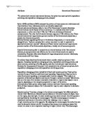
The Swan(1960) diagram depicts this very point, the diagram works under the following assumptions, a non existent international capital flow (so balance of payments = nations trade balance) and a constant price level(until aggregate demand begins to exceed the full employment level of output).
The vertical axis measures the exchange rate and the horizontal axis measures real domestic expenditures. All points along the EE curve refer to external balance, with points to the left and right indicating external surplus and deficits respectively. Points on the YY curve refer to internal balance, with points to the left indicating internal unemployment and points to the right indicating internal inflation. Where the YY and EE curves cross defines the four zones of external and internal imbalance and helps to determine the appropriate combination policy to reach both internal and external balance, represented above by point F.
The EE curve demonstrates the various combinations of exchange rates and real domestic expenditures that result in external balance. The EE curve is upward sloping; as a higher, devalued currency (R) would improve the nations trade balance (if the Marshall-Lerner condition is satisfied). Consequently there must be a corresponding increase in real domestic expenditures (D), to cause imports to rise sufficiently to keep trade balance in equilibrium and maintain external balance. For example, an increase in R, from R2-R3 will be followed by a increase in D, from D2-D3 in order for the economy to maintain external balance, represented by J. A comparatively smaller increase in D will lead to a balance of trade deficit. Alternately the YY curve demonstrates the various combinations of exchange rates (R) and domestic absorption (D) that result in internal balance.
The YY curve is negatively sloped as revaluation worsens the trade balance, and must be matched with a larger domestic expenditure (D), for the nation to remain in internal balance. A smaller increase in D will result in unemployment while a larger increase will result in demand-pull inflation.
It is from this diagram that we can determine the combination of expenditure-changing and expenditure-switching policies required to reach point F. for example from C, both absorption (domestic expenditures) and the exchange rate must be increased to reach equilibrium, F. By increasing R only the nation can achieve either external balance (C1 on EE) or with a smaller increase in R internal balance(C2 on EE), but it cannot reach both simultaneously. Likewise, by only increasing domestic absorption, the nation can reach internal balance (J on YY), but this leaves an external deficit on as it is below the EE curve.
If for example the nation were already in internal balance (J on YY), a devaluation of the currency could get the nation to point (J1), however in this case the nation would consequently face inflation. Thus, it is two policies that are usually used in order to achieve both goals simultaneously. Only if the nation is directly across from, or right above or below point F can the nation reach point F with a single policy instrument. For example, point N to F is available by increasing domestic absorption from D1-D2. This happens because absorption causes imports to rise, by the exact amount to eliminate the original surplus without a change in the exchange rate.
History dictates the economy. Thus, as the Second World War came to a close, industrial nations were unwilling to devalue or revalue their currency even when they were in fundamental disequilibrium. Surplus nations enjoyed the reputation of a surplus, but deficit nations regarded revaluation as a sign of weakness and consequently nations were only left with expenditure-changing policies to achieve both internal and external balance. This was a conundrum until Mundell demonstrated how to use fiscal policy to achieve internal balance and monetary policy to achieve external balance. Thus making it possible for nations to achieve both internal and external balance via the use of only one policy option.
To demonstrate the Mundell-Fleming model I must introduce a new diagram, and explaing the tools used in order to construct this model. The model below consists of three curves, the IS curve, showing all points at which the goods market is in equilibrium, the LM curve showing all points at which the money market is in equilibrium, and the BP curve, similarly showing equilibrium in the balance of payments. Short-term capital is now assumed to be responsive to international interest rate differentials. It is this response that allows the separation from fiscal and monetary policy, and consequently direct fiscal policy to achieve internal balance and monetary policy to achieve external balance.
The IS, LM and BP curves demonstrate the various combinations of interest rates and national income at which the goods market,money market, and the nations balance of payments are all in respective equilibrium. The IS curve is downward sloping as lower interest rates and higher investments are associated with higher incomes, and higher savings and imports, for the quantities of goods and services demanded and supplied to remain equal. The LM curve is positively inclined because higher incomes are associated with higher interest rates, and a lower demand for speculative money balances, for the total quantity of money demanded to remain equal to the given supply of money. The BP curve is also positively inclined as higher incomes and imports require higher rates of interest for the nation to remain in the balance of payments equilibrium. All markets are in equilibrium at point E, where the IS,LM and BP curves cross.
This model demonstrates how internal and external balance can be achieved via the use of expenditure changing policies only. Therefore I propose that single policy internal and external balance can be achieved in theory, but in practice it has been proved otherwise.
The early 1980s was a period of unstable economic conditions in developing countries. The aggregate current account deficit stood at $108.4 billion in 1981 up from $61.3 billion in 1979 (IMF, 1993). Inflation rates averaged at 20.4 percent in 1979-83, a significant increase from the 12.7 percent average in 1976-78. The average real GNP growth was 2.5 percent in 1979-83 down from 5.9 percent in 1976-78. These trends resulted from unfavorable domestic and external developments in the early 1980s. The exchange rates in many developing countries were overvalued. Fiscal policies were expansionary. The terms of trade of developing countries declined by 6.5 percent in 1980 and 4.9 percent in 1981. The world economy contracted in 1982. The London Interbank Offered Rates (LIBOR) peaked at 16.7 percent in 1981, the highest rate during the 1970s and 1980s.
To correct the macroeconomic imbalances, the World Bank and IMF with the support of many bilateral donors and other international financial institutions supported and financed the implementation of adjustment programs. These programs include the IMF stabilization programs, the aim of which is to achieve external and internal balance. However in practice many nations found these policies to underachieve without devaluation, thus I recommend a balanced use of both expenditure-switching and expenditure-changing policies.