- Measurement of the cross sectional area
To calculate the cross sectional area (c.s.a), it was necessary to measure both the width and the depth of the section of river. To measure the depth we worked out the D.S.I (depth sampling interval). Our group would collect a metre rule to measure the depth of the river. We placed a tape measure next to one of the ranging poles and then measured the distance between this pole and the other pole at the start line on the opposite bank, making sure that the tape measure was taut (see figure 5). We then divided this distance by a number and this gave us the D.S.I. We then measured the depth of the river at each evenly spaced point. We used the total distance between the two poles at the start line as the width of the stretch. Whilst doing this we took a few precautions. When placing the metre rule in the water, we made sure that it was straight, and that the end of the metre rule was touching the bed not touching large rocks or pebbles. This enabled us to make an accurate measurement.
-
Measurement of speed and depth across a meander
Once we had identified a suitable meander, that had a slip off slope, a river- Cliff and was shallow enough to work in, we began taking our readings (see figure 6).
We placed two ranging poles on the meander, one on the inner bank, the other on
The outer bank. We then measured the width between the two poles, using a tape measure. The two poles were both placed as close to the water’s edge as possible. Then we calculated the D.S.I by dividing the width by a suitable number. We measured the depth at each of these five points, which were evenly spaced between the two poles. We used a meter rule for this procedure, using the precautions listed earlier. The measurements were then passed to the data recorder. At each of our D.S.I’s we also measured the surface speed by using a flow meter (see figure 7).
- Measurement of sub-surface speed
To measure the sub-surface speed, we had to use a straight stretch of river, wide enough to give us a suitable number of readings.
Firstly we placed two ranging poles poles adjacent to each other on both banks of the river. Then we held a tape measure taut between the two ranging poles, and thus measured the width of the river, and then we calculated a width interval, by dividing the width of the river by a suitable number. At each width interval, we used a flow meter, placed under the surface, to measure the sub-surface speed.
Results
Table one ~ an overall class summary table of results
Table 2 ~ surface speed
Table three ~ c.s.a
Table four ~ Discharge
SUMMARY TABLE OF RESULTS
RIVER LEMON
STOP: GROUP:
BREAKDOWN OF BEDLOAD MEASUREMENTS
SUMMARY TABLE OF RESULTS
RIVER LEMON
STOP: GROUP:
BREAKDOWN OF BEDLOAD MEASUREMENTS
SUMMARY TABLE OF RESULTS
RIVER LEMON
STOP: GROUP:
BREAKDOWN OF BEDLOAD MEASUREMENTS
SUMMARY TABLE OF RESULTS
RIVER LEMON
STOP: GROUP:
BREAKDOWN OF BEDLOAD MEASUREMENTS
SUMMARY TABLE OF RESULTS
RIVER LEMON
STOP: GROUP:
BREAKDOWN OF BEDLOAD MEASUREMENTS
SUMMARY TABLE OF RESULTS
RIVER LEMON
STOP: GROUP:
BREAKDOWN OF BEDLOAD MEASUREMENTS
Introduction………………………………………………………. Page 1
Plates 1 & 2……………………………………………………….Page 2
Aims and methods……………………………………………...Pages 5-7
Results……………………………………………………….Pages 13-14
Explanation of results………………………………………..Pages 27-28
Conclusion………………………………………………………..Page 29
Appendices A………………………………………………Pages 30-41
Appendices B………………………………………………..Pages 42-44
Appendices c………………………….…………………… Pages 45-50
GEOGRAPHY FIELD TRIP – DARTMOOR 1999
DATA RECORDING TABLE
Flow conditions on ………………………… Date ………………
Site name ………………………………….. Group……………..
1. Velocity measurements:
Time in seconds for float to travel…………………………..Metres.
………….. , …………. , ………… , ………….. , ………….. ,
2. Width (m): ………… , ………….. , …………..
Average: ………….. ,
3. Depth sampling interval: …………… cms/ms
Average: …………………………..
4. Wetted Perimeter (m): ……………..
5. Bedload measurements (cms):
……,…...,…...,…...,…...,…...,…...,…...,…...,…...,……,……,…...,…...,……,
6. Flood Plain measurements:
Left bank………………………(m) Right bank……………………….(m)
7. Field Sketch:
GEOGRAPHY FIELD TRIP – DARTMOOR 1999
DATA RECORDING TABLE
Flow conditions on ………………………… Date ………………
Site name ………………………………….. Group……………..
1. Velocity measurements:
Time in seconds for float to travel…………………………..metres.
………….. , …………. , ………… , ………….. , ………….. ,
2. Width (m): ………… , ………….. , …………..
Average: ………….. ,
3. Depth sampling interval: …………… cms/ms
Average: …………………………..
4. Wetted Perimeter (m): ……………..
5. Bedload measurements (cms):
……,…...,…...,…...,…...,…...,…...,…...,…...,…...,……,……,…...,…...,……,
6. Flood Plain measurements:
Left bank………………………(m) Right bank……………………….(m)
7. Field Sketch:
Explanation of Results
Our hypotheses stated that the fastest flow of water on a straight section is in the middle however at Haytor my group’s results of the float travelling 2.30 metres, placed at regular intervals across the width of the river did not show significant increase in speed in the central flow. The water appeared to flow fastest on one side of the river (12.12, 10.95 seconds) with the slowest speed in the middle (13.52 seconds).
At Pinchaford farm the float travelled 2.05 meters and my results showed that the fastest flow was on one side of the river (12.75 seconds) with the central recording having the 2nd fastest flow. There did not appear to be a significant flow pattern. This may have been due to the effects of a mini-waterfall along this stretch of river and tree branches submerged on the water surface.
At Bickington the results showed medium flow of the water nearest the banks. The slowest flow was in the middle with the faster flow (28 seconds) was between the side and the centre. The float had to travel 8.70 metres, which would explain the longer time in seconds, than at previous stops.
At Chercombe Bridge the float travelled the longest distance, so far, of ten metres. Once again the fastest speed was recorded at either side of the river. The slowest speed was recorded in the central flow.
At Bradley Manor the fastest flow was towards one side with the slowest flow on the opposite side. There did seem to be a definite flow pattern across this section of river. The field sketch indicated that there were larger rocks on one side of the riverbed (with the slowest flow) and smaller pebbles on the side with the faster flow.
We measured the depth at regular intervals across the width of the river at each site. We analyzed the data to see if the deepest part of a straight section occurred in the middle.
At Haytor the river was very shallow and very narrow, however the deepest part was towards the middle.
At Pinchaford Farm the deepest part of the river was not in the middle but towards one of the sides as shown in the profile.
At Bickington the river bed was unlevel, however the deepest part was towards one side, as again shown in the profile.
At Chercombe Bridge the depth sampling interval gradually began to increase to 90 cm and the deepest part of the straight section was in the middle.
At Bradley Manor the depth sampling interval was the largest at 100 cm, however the deepest part was towards one side.
We investigated the water flow of a meander at Mallands. We used our group’s data to make a scatter graph (figure 8) and this clearly showed that the water flowed faster on the outer-bank. The fastest speed was 0.89 m/sec. The slowest speed on the inner bank was 0.05 m/sec. This showed an increase of 0.84 m/sec towards the outer-bank. The last reading on the edge of the outer-bank of the river showed a decrease of 0.38 m/sec.
The profile of a meander (figure 9) showed the depth gradually increases towards the outer-bank, which supports the hypotheses stated earlier. The slower water flow on the inner bank allows for the deposition of material on the river bed. The faster flow causes more erosion and therefore creates deeper water towards the outer-bank.
We investigated that the fastest sub-surface current is in the middle and just below the surface. The water around the banks, bed and surface will have the most friction so the part of the river in the middle will have the most friction free water. Therefore the middle will flow much faster than the outside parts (near to the bed, banks and surface). Our results in figure 14 supports this theory. The fastest speed was between 0.21 and 0.30 m/sec which was in the middle and just below the surface. The slowest speed was nearest the bank and the river bed and was between 0.01 and 0.10 m/sec.
Conclusion
I set out to test my all of my five hypotheses and calculate accurate results. I achieved all that I planned to do and my results were more or less what I expected.
I benefitted from the exercise because it taught me many things about rivers that I had not thought about. The habitat around the area we were working in was quite varied and gave us a contrasting location compared to the outskirts of London where I live. It was my first trip of this kind and I gained a lot of experience on how to make accurate measurements and how to conduct fieldwork. I also learnt to expect the unexpected. The exercise also allowed me to put into perspective, some elements of hydrology. For example: the size and scale of a meander.
The results did not always tally with what I had been taught in the classroom, because we only studied the river in late summer and therefore the river flow might have been lower than average. If the river was more easily accessible, I would have liked to repeat the investigation several times over a number of months to give a seasonal comparison. But still, I saw many features of the river that I would not have seen anywhere else like the mini-waterfall at Pinchaford farm where I tested my hypotheses.
The instruments we used in the investigation were not too difficult to use, however if the river was running quickly, the flow meter was giving problems as we had to keep it steady to record the measurements.
The exercise required us to perform as a team; this meant that we had to form a group (six in all) consisting of four or five members. Each group had to nominate a leader who was responsible for organizing the group and overseeing each activity at each stop. We also had to decide on a reliable data recorder who had to be fast and accurate in order that we would have a reliable set of results.
Illustrations
Page 2 – Photograph of Longlands Field Study Centre
Page 2 – Photograph of view from top of Haytor rocks
Page 7 – Photograph of Chercombe Bridge
Plate 1-Longlands Field Study Centre
Plate 2-View From Top of Haytor Rocks