4 Theoretical Background:
-
Corrasion, also known as abrasion, is the grinding of rock fragments transported by the river against the bed and banks of the river. Corrasion happens both vertically and laterally. (Nagle G. (2000) Advanced Geography. 2nd ed. Oxford: Oxford University Press.)
-
Attrition is the colliding of rocks in the water against one another. The fragments are therefore broken into smaller pieces and become smoother and rounder along the process. (Nagle G. (2000) Advanced Geography. 2nd ed. Oxford: Oxford University Press.)
-
Solution, also known as corrosion, is when the river water reacts chemically with materials and sediment in the river and manipulates its shape and size. (Nagle G. (2000) Advanced Geography. 2nd ed. Oxford: Oxford University Press.)
-
Hydraulic action is the breaking down of rocks and dragging them away from the bed and banks by the force of the running water itself. When water from a fast moving stream enters cracks in a rock, the force breaks up the force into pieces. (Nagle G. (2000) Advanced Geography. 2nd ed. Oxford: Oxford University Press.)
-
Discharge increases, because water is added to the stream from tributaries and groundwater. As discharge increases, width, depth, and velocity of the stream increase. The gradient of the stream, however, will decrease. (Nagle G. (2000) Advanced Geography. 2nd ed. Oxford: Oxford University Press.)
-
Bedload - coarser and denser particles that remain on the bed of the stream most of the time but move by a process of saltation as a result of collisions between particles and turbulent eddies. Note that sediment can move between bed load and suspended load as the velocity of the stream changes. (Nagle G. (2000) Advanced Geography. 2nd ed. Oxford: Oxford University Press.)
-
Velocity will be distributed according to the position of the flow. (Nagle G. (2000) Advanced Geography. 2nd ed. Oxford: Oxford University Press.) It will depend on factors such as:
- Channel Roughness
- Channel Slope
This is clearer to see from the example below:
Figure 4.1: A diagram which shows an example of where the areas of different velocities can be found in a cross-section.
http://www.benthos.net/images/Vienna%20International%20School/River%20Coursework/Channel%20Velocities.jpg
5 Data Collecting Methods:
Whilst it would be quite a difficult task making accurate measurements of characteristics such as: channel slope, roughness of bedload, etc., accurate measurements of characteristics such as: velocity, depth, and bedload size and angularity were able to be made.
Firstly, a laser was set up, balanced and pointed accross the river to be able to aquire an accurate bankful level, which would make all other measurements of depth simple. A string was then spanned from where the laser-pointer was situated to where it pointed, and then it was tied to a tree. The laser was an extremely useful item because operating it was fairly simple and it was a lot more accurate than most older methods. After that was accomplished, a tape measure was spanned accross the river from exactly where the string started to where it ended.
It was then possible to collect data every 25 cm. This would allow more data to be collected so that the results would be more likey to prove or disprove theories. A greater distance would have made results more inaccurate but therefore less time-grasping. A shorter distance would have shown the opposite.
The entire data collecting took place in 4 large locations progressing downstream. Due to the minor water level in location 1, it was impossible to accumulate appropriate depth, length, and velocity readings.
The locations that were to be examined where very appropriate because they were easily accessible and also an adequate length apart from eachother so that it is possible to get a clear view on how the river behaves, progressing downstream.
Width and Depth
Since the river was too shallow for acceptable measurements, locations 2-4 were measured. As previously mentioned, a tape measure was set up and used to measure the distance accross the river. After the lateral measurements had been aquired, vertical measurements were taken using a long ruler and measuring the distance between the ground and string every 25 centimetres, using the tape measure as a guide. This information was gathering entirely accross the stream, until about 50 centimetres after the last water depth was recorded. This water depth was also very useful, because the previous depth measurements were only valid for the depth of bankful. The equipment used in this method led to positive results because everyone was familiar with the tools and therefor caused no complications.
Velocity
Once again, the stream at location one was too shallow, therefor velocity readings could only be recorded at locations 2-4. In these locations, a velocity meter was held into the water every 25 cm at about 1/3 the water depth (by theory, this is the area of highest velocity). The meter was placed in the water for 6 seconds and the number of rotations were counted. Logically, to get the number of rotations per minute, it was simply necessary to multiply the figure aquired by 10. This method, using the velocity meter was very easy to understand and proceed with.
Bedload
At each location 30 samples of bedload were assembled and measurements were taken using a caliper. Three dimensions of the bedload sample were measured; length (A), width (B), and depth (C). Then adding all these values up it was possible to come up with a total value. Using a scale from 1-6, its angularities were observed and then categorised (These different categories are called classes and the raw data sheet can be viewed under Data Presentation: Location 1 on page 15). The caliper was used because it could provide very accurate measurements. The amount of samples used was adequate because it provided enough information to get a good image of what the average bedload was like in a certain region.
Figure 5.1: Diagram on Bedload and a suggested method on Measuring it.
6 Data Presentation
Location 1
Description
Location 1 was the area where the spring was. On the western side of the stream there are tall mountains with lots of beech and carnivorous trees, the other side has several trees aswell, but not nearly as many as on the other side due to the natural catastrophe. There are many large angular boulders, which would indicate that these have fallen of the mountain quite recently. There is an underground water supply from where the river springs up, and simply looks like it is flowing out of the rocks. There are extremely many rocks, very angular and of all sizes, and many broken branches.
Figure 6.1 – On the left side of the photo it is possible to see an area very near to the “ursprung” because of the size of the stream. Further on the right hand side, the stream has become much wider already.
Location 1 Graphs
Location 2
Description
Location 2 is fairly further down the stream from location 1, because the waterlevel has already risen to a level where accurate velocity readings can be aquired. Not only has the depth increased since location 1, but also the width. Once again there is a lot of vegetation on both sides, with mainly deciduous trees. The mountain side still remains but it is difficult to see through the thickness of trees (figure 5.2). One side of the river stops instantly and has a drastic increase in bankful depth. On the other side there is a pebbly beach, which extends about 5 meters up to the forest. The area beyond that is fairly flat aswell whereas on the other side there are many boulders and drastic increases in height.
Figure 6.2 – In the foreground it is possible to see the long steady bank whereas in the background shows a drastic increase in height with rocks and a forest.
Location 2 Tabular Data
Location 2 Graphs
Location 3
Description
As on the previous locations, there is dense vegetation on both sides of the rivers. On the side of the valley the bank is quite swampy and sandy. On the other side, the mountain side, there is once again mainly deciduous forest. The banks are fairly broad and do not drastically increase in height as in location 2. The river at location three is the widest. Beyond bankful there are mainly gravel and pebbles, but until then the banks consist of mud and sand.
Figure 6.3 – In the foreground it is possible to see big boulders and the background shows the pebbly beach.
Location 3 Tabular Data
Location 3 Graphs
Location 4
Description
At location 4 the stream was fairly thinner but yet deeper than at location 3. In Figure 5.4, it is obvious to see that one bank of the river drastically increases in height. This is because it is a man-made bank to avoid flooding the cattle field which is beyong that. The other bank seems quite natural and constists of pebbles, gravel, and fallen leaves. The trees at this location are mainly deciduous but there are some beech trees. At the end of location 4, there is a man-made waterfall, whos purpose is not known.
Figure 5.4 – On the left it is possible to see the man-made bank covered with few trees. The right shows part of the forest and the pebbly beach covered with leaves.
Location 4 Tabular Data
Location 4 Graphs
7 Data Analysis and Discussion
Location 1
Since the only variable that was measured at location 1 was Bedload Angularity, it is the only data for Location 1. The most common bedload type found at this location was class 1: “very angular”. Several others were found as well, but these were all angular.
Table 7.1 – This table shows how many bedload samples of each class were collected at Location 1
Location 2
All possible Data was collected for Location 2 so it is possible to calculate various important factors:
NOTE: These results are those of the current water level and not of bankfull.
Hydraulic Radius
Following the theory that “HR = area/wetted perimeter” (Nagle G. (2000) Advanced Geography. 2nd ed. Oxford: Oxford University Press.).
Area = 9,75 m²
Wetted Perimeter = 7,00 m
Hydraulic Radius = 1,35 m
Discharge
Since the Cross-Sectional Area is already calculated, it is simple to find out the discharge. The theory that is involved here is that “Discharge = area*average velocity” (Nagle G. (2000) Advanced Geography. 2nd ed. Oxford: Oxford University Press.)
Area = 9,75 m²
Average Velocity = 0,82 m/s
Discharge = 8,28 cumecs
Spearman’s Bedload/Velocity Rank Correlation – Location 2
Table 7.2 – This table shows all the data that is necessary to calculate Spearman’s Rank correlation for bedload and velocity
Graph 7.3 – This graph shows the correlation between bedload size and velocity. It is clear that the correlation is positive in this instance.
Spearman’s Depth/Velocity Rank Correlation – Location 2
Table 7.4 – This table shows all the data that is necessary to calculate Spearman’s Rank correlation for depth and velocity
Graph 7.5 – This graph shows the correlation between depth and velocity. It is clear that the correlation is positive in this instance.
Location 3
All possible Data was collected for Location 2 so it is possible to calculate various important factors:
NOTE: These results are those of the current water level and not of bankfull.
Hydraulic Radius
Following the theory that “HR = area/wetted perimeter” (Nagle G. (2000) Advanced Geography. 2nd ed. Oxford: Oxford University Press.).
Area = 11,00 m²
Wetted Perimeter = 7,75 m
Hydraulic Radius = 1,41 m
Discharge
Since the Cross-Sectional Area is already calculated, it is simple to find out the discharge. The theory that is involved here is that “Discharge = area*average velocity” (Nagle G. (2000) Advanced Geography. 2nd ed. Oxford: Oxford University Press.)
Area = 11,00 m²
Average Velocity = 0,72 m/s
Discharge = 4,4 cumecs
Spearman’s Bedload/Velocity Rank Correlation – Location 3
Table 7.6
Graph 7.7
Spearman’s Depth/Velocity Rank Correlation – Location 3
Table 7.8
Graph 7.9
Location 4
All possible Data was collected for Location 2 so it is possible to calculate various important factors:
NOTE: These results are those of the current water level and not of bankfull.
Hydraulic Radius
Following the theory that “HR = area/wetted perimeter” (Nagle G. (2000) Advanced Geography. 2nd ed. Oxford: Oxford University Press.).
Area = 9,50 m²
Wetted Perimeter = 9,00 m
Hydraulic Radius = 1,06 m
Discharge
Since the Cross-Sectional Area is already calculated, it is simple to find out the discharge. The theory that is involved here is that “Discharge = area*average velocity” (Nagle G. (2000) Advanced Geography. 2nd ed. Oxford: Oxford University Press.)
Area = 9,50 m²
Average Velocity = 0,72 m/s
Discharge = 6,84 cumecs
Spearman’s Bedload/Velocity Rank Correlation – Location 4
Table 7.10 – This table shows all the data that is necessary to calculate Spearman’s Rank correlation for bedload and velocity
Graph 7.11 – This graph shows the correlation between bedload size and velocity. It is clear that the correlation is negative in this instance.
Spearman’s Depth/Velocity Rank Correlation – Location 4
Table 7.13 – This table shows all the data that is necessary to calculate Spearman’s Rank correlation for depth and velocity
Graph 7.14 – This graph shows the correlation between depth and velocity. It is clear that the correlation is positive in this instance.
Graphs and Data relating to all Locations
Average Bedload Angulariy
The unit that is used in the following graphs and tables is the class of bedload angularity. View method for more details on bedload angularity classification (the raw data sheet can be viewed under Data Presentation: Location 1 on page 15).
Table 7.15 – Tabular Data of the average bedload angularity of each location
Graph 7.16 –A barchart showing the increasing average bedload angularity
Graph 7.17 – A web diagram showing the distribution of average bedload angularities among all locations.
Average Bedload Size
The unit that is used in the following graphs and tables is the total size of bedload (measurement A+B+C).
Table 7.15 – Tabular Data of the average bedload angularity of each location
Graph 7.18 – A barchart showing the decrease in average bedload size as the locations progress down the river.
Graph 7.19 – A web diagram showing the distribution of average bedload size among all locations.