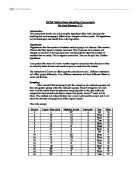
Sampling:
I shall use stratified sampling to split the categories into instructor groups and then into gender groups within the instructor groups. These 8 categories will each have ¼ of the results taken by systematic sampling (after all the data within the category has been sorted according to lesson time spent); every 4th result will be taken. This method will reduce the data into a more easily useable sample and it will retain the diversity and proportion of the original results.
This is the sample
Presentation and Analysis
The results will be displayed on scatter graphs to show the correlation and will be equipped with a line of best fit and correlation coefficient (worked out on excel). This will show the correlation strength (1 – strong positive and -1 is strong negative).
This graph shows the whole sample for lesson time against no. of mistakes. The correlation coefficient of - 0.47 indicates significant negative correlation and supports my hypothesis (mistakes go down as time goes up).
Graph for females. This shows weaker negative correlation (- 0.27) Females, have a weaker correlation than males. This opposes my hypothesis.
This graph, for males results, shows stronger negative correlation (- 0.58) than with females. This opposes my hypothesis. However, both males and females show negative correlation or the same reason as predicted.
his shows the results with instructor A. – 0.86 shows a strong negative correlation. This means that instructor A is a fairly constant and effective teacher.
This graph shows instructor B results and with a corrl coeff of – 0.46 a much weaker –ve correlation is shown. This is half of inspector A and this implies that B is approximately half as effective a teacher as A (in terms of consistency).
The correlation coefficient of - 0.95 is very strong (close to perfect) and shows that instructor C is the most effective instructor yet (mistake no. is reduced with increasing lesson time at the fastest rate).
Instructor D shows the same correlation (- 0.87) approx as A. H/she is clearly an effective instructor on account of high negative correlation (rate of decrease in mistakes is high against time spent).
Inst A, females.
-0.91
Inst A, males,
-0.83
These 8 graphs show instructors with different genders. The correlation coefficient is displayed next to each. The former graph on each page is for females and the latter is for males. The graphs begin with instructor A and go through to D.
Inst B
females
- 0.01
B males
-0.84
C, female
0.99
C, male
- 0.91
D, female
0.91
D, male
0.86
Conclusion:
As the number of hours spent on lessons increases, the no. of mistakes decreases because the people become better drivers.
Females show weaker correlation than males; this implies that they are less affected by the lessons. This disagrees with my hypothesis and proves it wrong.
Different instructors show different correlation. The order of correlation strength and effectiveness as a teacher (from most to least) is as follows: C,D,A,B. All instructors show a roughly equal effectiveness on males and females except B. Instructor B shows far weaker correlation with females than males, he is more effective when his/her students are male.
Evaluation:
There was an insufficient data amount to conclude definitely on the last few graphs (instructor and gender). But other than that, all went well. Valid and easily identifiable conclusions could be drawn.