Despite the fact that the linear programming technique can be applied in a variety of different problems there are unfortunately some disadvantages that we should take into consideration before using this method.
The Linear programming method assumes constant return to scale, which implies that outputs are thus exactly proportional to inputs. Doubling all inputs doubles outputs and doubles cost, and so on.
A second disadvantage is that linear programming may also
yield a non-integer solution and therefore may give unrealistic results or outcomes to the problem.
However, it is sometimes possible for two special cases to arise when we attempt to solve linear programming. These special cases can be considered as additional disadvantages or limitations for the linear programming technique. The first instance is the case where no feasible solution to the linear programming problem is suitable for the entire constraints. This problem is referred to us as infeasibility. Infeasibility can arise due to management’s high expectations or due to too many limitations that have been placed on the problem. The second case is where the solution might be unbounded. This means that the value of the solution to maximization or minimization problems is infinitely large or small respectively, without violating any of the constraints. For the unbounded result, management has to change the objective function to find a more realistic solution.
Finally linear programming makes two simplistic assumptions. Firstly it is deterministic which means all inputs are fixed and therefore under the full control of the decision maker (complete certainty). In reality a stochastic model would be preferable because for example production time per unit may be influenced by environmental factors, and subject to variation (uncertainty). Secondly the model is additive which means that the value of the objective function and the total resources used can be found by summing the objective function contribution and the resources used for all decision variables.
(b) (i) Formulate this problem as a linear programming
X= number of cows Y= number of pigs
MAXIMISE: 40X +20Y
Constraints:
(1) 3X+Y ≤ 9
(2) X+Y ≥ 4 X, Y ≥ 0
(3) X ≤ 4
(4) Y ≤ 6
Series 1
3X+Y=9
IF X=0 therefore Y=9 Point:(0,9)
IF Y=0 therefore X=3 Point:(3,0
Series 2
X+Y=4
IF X=0 therefore Y=4 Point:(0,4)
IF Y=0 therefore X=4 Point:(4,0)
Series 3
X=4
IF Y=0 therefore X=4 Point:(4,0)
IF Y=10 therefore X=4 Point:(4,0)
Third equation is a parallel straight line to the y-axis
Series 4
Y=6
IF X=0 therefore Y=6
IF X=5 therefore Y=6
Fourth equation is a parallel straight line to the x-axis
First
Graphical representation:
Suppose that the maximum profit is £200
then the objective function would be :
O.F. 40X+20Y=200
When X=0 then Y=10 Point (0,10)
When Y=0 then X=5 Point (5, 0)
When the profit is equal to £200 the iso-profit curve (40X+20Y=200) is displayed above all 4 budget constraints. Therefore the iso profit curve is shifted south-west, parallel to itself, until it hits the highest point of an intersection between two budget constraints in the feasible region. This point is the number three in the figure above. The optimum point is (1, 6) .That means 1 cow and 6 pigs. The maximum profit line which hits the feasible region at its optimal point is 40X+20Y=160 .The representation of this situation is displayed in the second graphical illustration
Second
Graphical representation:
Optimum point: intersection of series (1) and (4)
(1) 3X+Y=9
(4) Y =6
Solve the two equations simultaneously
3X+Y=9 (1)
Y=6 (4)
Equation 4 in 1: 3X+6=9
3X=3
X=1 (1, 6) Optimal Point
Substitute this point in the objective function: 40X+20Y
Maximum profit 40*1+20*6=160
Dual or shadow prices
We are choosing the constraint number 1 and the constraint number 4 because they have positive dual value in a change of a bushel or a pig respectively. A change in bushel or pig causes changes in profit. The second and the third constraints have zero dual prices; increase on their resources won’t affect profit.
Therefore: if we increase the number of bushels by one at the right-hand side of the first constraint then 3X+Y=10
and Y =6
equation 4 into 1:
3X+6=10
X=4/3 , Y=6
Plugging into the O.F: 40*(4/3) +20*(6) = £173⅓ Dual price for increase or decrease of bushel by 1 is £13⅓
--------------------------------------------------------------------------------------------------
Now increase of 1 pig at the right-hand side of the fourth constraint
Y=7
and 3X+Y=9
equation 4 into 1
3X+7=9
X=⅔ , Y=7
Plugging into the O.F: 40*(⅔) + 20*(7) = 166⅔
Dual price for an increase or decrease of a pig is £ 6⅔
Shadow price and dual price are exactly the same for all maximization linear programs. The economic meaning of shadow prices is very important for the managers. Shadow price is the changes in profit (positive or negative) of a marginal increase of scarce resources in any of the constraints in the linear programming procedure. Therefore the managers can gather information from the performance of each constraint and give emphasis to an increase of those resources with the highest opportunity cost or shadow price. In our case it would be beneficial, and more profitable for the farmer to increase the number of the bushels rather than the number of pigs to achieve a greater profit.