When getting to grips with statistical notation it is important to remain un-intimidated. Mathematicians are not cleverer than everyone else. They just speak another language. All you need do is learn enough of a smattering of mathematical language to bluff your way in statistics textbooks. This is likely to require hard work rather than super-human intellectual powers.
Averages: mean, median and mode.
The mean is the “normal” average.
The median is the middle value, it is the central value of the n observations when placed in numerical order. If there are an odd number of observations it is while for an even number it is . It should be clear that the median need not be one of the x values. This value is often used when one or two extreme x values distort the mean.
The mode is the most commonly occurring value and would be of importance to a manufacturer when assessing what style of product to market.
Averages are normally taken to be representative of a larger set of data, but data with the same average can differ in lots of other ways. For example, these data have the same mean.
Fig. 1
Two graphs showing very different data sets that share the same mean. In the right hand graph, values tend to be close to the mean, while in the left hand graph, values tend to be further from the mean. The left hand graph shows values that are move variable (see next lecture).
The following data have the same median.
Fig. 2
Two graphs showing very different data sets that have the same median. The left hand graph shows data that is symmetrically arranged around the median (and mean). The right hand graph shows “negative skew”, where values below the median are further from the median than values above the median. In the right graph, the median and the mean will have different values.
The following data have the same mode.
Fig. 3
Two graphs showing very different data sets that have the same mode (or modal average). In neither case is the mode a very good summary of the data.
Introduction to equations and statistical notation
The symbols discussed in the lecture are “sigma” (the summation symbol, Σ), “mu” (population mean, μ), “X bar” (sample mean, ), “xi” (the ith value), “n” (number of values). See any introductory text for a basic introduction to statistical notation.
Definition of the mean
The arithmetic mean is the sum of the values divided by the number of values. This is shown below using mathematical notation. It is best to get to grips with the symbols while the statistical concepts they represent (e.g. mean average) are simple and familiar.
Sample mean vs. population mean
μ, the population mean, is the mean derived from the entire population under study. Population is a word with a somewhat elastic meaning, but generally it is up to you, the experimenter, to define your population. It might be all the people in the UK, all the people who shop at KwikSave, or all the lecturers in the Newcastle University Psychology Department. With large populations, it is often impractical to find μ.
, the sample mean, is calculated from a representative sample of the population. This is usually done by selecting individuals from the population at random to avoid sampling bias. You get sampling bias when all the members of the population under study do not stand an equal chance of being measured.
If you wanted to estimate the mean height of people in the UK, it would be stupid to do all your measuring in primary schools. This is an extreme example, but more realistically, suppose you wanted to get a representative 1000 people to complete a questionnaire on social attitudes. If you did the survey by telephone, your sample would be biased towards telephone owners. If you called between 9 and 5, your sample would be biased towards people without day jobs. If you did the survey in high streets, your sample would be biased towards town dwellers, who were out shopping during the day, who were friendly, and who had enough time to talk to someone in the street with a clip-board etc. etc. Sampling bias is a real problem in much research in psychology and the social sciences.
Even if you manage to avoid sampling bias, is unlikely to be exactly the same as μ. On average, however, the larger the sample then the more likely it is that will be close to μ. This is why polling organizations have to ask hundreds (or thousands) of people if they want to be reasonably confident of getting that is within a few percent of μ.
To illustrate this point, I made a large population of numbers with a mean of 100.0 (μ = 100.0) and a standard deviation of 15 (standard deviation is a measure of spread from the mean and we will discuss it in greater detail later in the course). I then took 40 samples of 5 numbers and 40 samples of 20 numbers from the population. The means of the samples () are presented below.
Fig 4.
The stem and leaf plot shows the distribution of the sample means () of samples taken from a population with a mean of 100 and a standard deviation of 15. The individual sample means may be obtained from the plot by adding the value in the left hand column (e.g. 90) to values in one of the boxes. For example, with the sample size of 5, samples had means with 81, 86, 92, 93, 93, 94, 94, 94, etc. It is clear that the small sample size results in a greater spread of values for .
Estimating the mean from a bar chart of frequencies
Fig. 5
It is possible to estimate the mean from a frequency bar chart (e.g. above). “n”, the number of scores, can be calculated by adding up the heights of all the columns. The sum of all the scores can be calculated by multiplying each of the column heights by the x-axis midpoints. The mean is then simply the estimated sum of scores divided by n.
How representative is the mean?
Sometimes, it might be useful to be able to measure how well the mean fits the data that generated it (e.g. Fig. 1). At first sight, one might think that it would be possible to find the total of the difference between each score and the mean. Unfortunately, this approach will not work. By definition, the sum of negative differences (from scores less than the mean) will exactly cancel out the sum of positive differences (from scores that are greater than the mean). The sum of deviations from the mean is always zero.
Sum of Squared Deviations
Positive and negative deviations from the mean cancel out when you sum them. Squaring the deviations before summing is a mathematical trick to turn negative deviations into positive “squared deviations”. Why is this important? The graph below illustrates the answer.
Fig. 6
To assist with the interpretation, the charts are plotted side-by-side. Note that identical axis have been adopted.
A bar chart showing two samples with the same mean (0). The right hand bars in each category represent a sample with a bimodal distribution (lots of low values and lots of high values) while the left hand bars in each category represent a sample with a peak frequency around the mean. The equation shows how the sum of squared deviations is calculated. The bimodal sample has a ss = 51882 and the unimodal sample has a ss = 9826; the sum of squared deviations from the mean is around 5 times greater for the bimodal distribution. Therefore, the mean is a much less accurate representation of the bimodal sample than it is of the unimodal sample.
The Median.
The median is the value that divides the distribution of values exactly in half. To find the median, sort or rank the values and find the middle value (if there are is an odd number of values) or else the mean of the central two values (if there is an even number of values). It is possible to estimate the median from histograms. Use the information on number of scores to estimate the position of the middle score.
Fig. 7
Estimate the position of the “middle person” on the income axis using the information on the frequency axis. Here there are 18 lecturers, so the median income is at the estimated position between 9 and 10. This is simpler to estimate from a cumulative frequency polygon.
The median average can be more representative than the mean in skewed distributions (e.g. annual income, or National Lottery winnings). Remember to look at the data when you calculate the median average
Fig. 8
The Mode
The mode is the score or category that has the greatest frequency. The modal average can be used with nominal data. As with all other averages, look at the data when you calculate the mode.
Fig. 9
Is a three dimensional representation sensible?