Our evidence is from the sample
What is the hypothesis in this example?
We are investigating a possible relationship between PACKAGES and TYPE
We are asked to test the statement that the acceptance of package customers is associated with hotel type, and we adopt this as our null hypothesis.
Unrelated is always the null hypothesis
What is the formal null hypothesis for this example?
H0:
What is the alternative hypothesis?
If the statement is not supported by the sample data then the acceptance of package customers pattern will be different from hotel type to hotel type, there will be evidence of a relationship and using the table we will be able to describe the relationship in more detail.
Related is always the alternative hypothesis
What is the formal alternative hypothesis for this example?
H1:
The Chi-Squared Test of Significance
To test the hypotheses, we calculate the value of the chi-squared ( χ2 ) statistic which is a single measure of the differences between the observed counts and the expected counts across all the cells of the table.
The questions to be answered are:
Do the expected cell counts and the observed sample counts differ by more than chance or random sample error?
Does the data ( observed sample cell counts ) exhibit random variation or a pattern of some type due to the presence of a relationship between the two variables?
You are not expected to reproduce the formula for the chi-squared statistic but it is useful to know how SPSS computes its value. The calculation is completed as follows:
χ2 =
- calculating what the expected count would be, if there were no relationship
between the two variables ( using probabilities )
- calculating the difference between the expected and observed cell counts for each cell
- squaring these differences
- adding the squared differences together
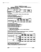
Accepts package tours * Type of Hotel Crosstabulation
χ2 Calculation:
Small differences between observed and expected produces a small contribution to the χ2 statistic
Large differences between observed and expected produces a large contribution to the χ2 statistic
SPSS calculates the value of the χ2 statistic for us:
Chi-Square Tests
Making a decision:
In effect the null hypothesis is presumed innocent until proven guilty
We require a decision rule to help us to test the hypothesis we have stated
The decision rule
We set up a decision rule - detailed explanation of the theory behind the use of this rule will not be discussed on this module. It will be used as a methodology for determining the existence of a relationship when you are unsure and no more.
There are many chi-square distributions. The one used is determined by degrees of freedom.
Degrees of freedom are actually calculated using the following formula
df = ( no. of rows in the table - 1 ) ( no. of columns in the table - 1 ) = ( 2- 1 )( 4-1 ) = (1)(3) giving 3df (but the SPSS output calculates the df for you)
DIAGRAM OF CHI-SQUARED DISTRIBUTION and DECISION RULE
The 95% decision point or the critical value is taken from pre-printed chi-square tables using the degrees of freedom (df) given.
Using the tables provided, what is the critical value for this example?
Applying the decision rule
It is unlikely that we will get a value of the test statistic in the 5% region.
Given that a value lying in the 5% region is very unlikely, we shall reject the null hypothesis if the value of the chi-squared statistic calculated from the sample data falls in this region.
What is the value of the χ2 statistic calculated by SPSS from the sample data? (see SPSS output)
If the value of our test statistic falls inside the 5% region on the diagram
reject H0: in favour of the alternative hypothesis
i.e. on the basis of the sample data there is a relationship between the two variables
If the value of our test statistic falls inside the 95% region on the diagram
we do not reject H0:
i.e. on the basis of the sample data, there is no relationship between the two variables
Analysis Conclusion
Strength of the relationship
Type 1 and Type 11 Errors
Hypothesis testing is not foolproof!
It is possible to make an error but it obviously would be bad luck if we did considering the small number of instances of a value in this region
Statistical Hypothesis Testing is a reasonable decision procedure in the face of two types of unavoidable ignorances
a) we will never know the truth
- we will never know whether our decision is correct or incorrect
CHI-SQUARED OUTPUT OF PACKAGES and TYPE
SPSS for Windows
Get the HOTELS data file
Select Analyze
Select Descriptive Statistics
Select Crosstabs
Move the variable Accepts package tours (packages) into the Rows box
Move the variable Type of Hotel (type) into the Columns box
Select Statistics button at the foot of the window
Select Chi-square
Select Continue
Select Cells button at the foot of the window
Select Expected in the counts box to give the expected frequencies.
Select Column in the Percentages box to give the column percentages
Select Continue
The OK to get the required output.
Lecture 7 - MG2007 Data Analysis
Plotting combinations of variables - categorical & measured
The Car Ownership Study
Objective 1 IDA Plan
Meeting the survey objective
Analysis - Number of Cars and Education in Years
( Box 2 of the IDA Matrix – Categorical RV/Measured factor )
Investigating the relationship between the number of cars a respondent owns and the education of household head in years
Univariate analysis ( SPSS commands - Frequencies or Explore )
Select the appropriate analysis for the data types of the RV and the factor
Bivariate analysis
We are interested in the distribution of the measured factor for each group of the categorical RV. Measured factor is the one with the associated distribution.
Is the mean number of years in education higher for those with two cars?
Is there a significant difference in the means between the two groups?
Distributions and relationships
A clear relationship means are same means are different
Clearly no relationship means are same means are different
Example questions to be asked
What is the mean number of years in education for the group owning 1 or less cars? How spread are the values for number of years? The S/D? The minimum and maximum values?
What is the mean number of years in education for the group owning 2 or more cars? How spread are the values for number of years? The S/D? The minimum and maximum values?
Possible outcomes of the analysis
There are three possible outcomes to the analysis at this stage:
there is an obvious relationship
there is obviously no relationship
there maybe a relationship
often difficult to be sure about a relationship and therefore we need to embark on further analysis
in the case of categorical RV/Measured factor, following comparison of means further analysis involves either t-testing or oneway analysis of variance dependent on the number of categories for the categorical variable
The Credit Survey
A Scenario
A retail company operates a number of different retail outlets across a number of regions in England and offers payment by credit in each of its stores. The company wishes to undertake an investigation into the nature of its credit transactions. In particular to investigate the factors associated with customers who pay using credit facilities, with the aim of building a profile of the customers using these facilities. This customer profile can then be used to develop a marketing strategy for the credit facilities aimed at a defined target group.
Available company records for customers who had obtained credit in 1993 provided the following data ( saved as Credit.Sav ) for the initial investigation.
Initial amount borrowed Actual amount (£s)
Declared Salary Actual amount (£s)
Age in years
Owner Occupier Coded 0 Owner Occupier
- Not an Owner Occupier
Region Coded 1 South West
- South East
- London
- Midlands
5 North
Objective 1
To investigate the factors associated with the amount customers borrow on credit
- Investigating relationships
Meeting the survey objective
Analysis – Amount Borrowed and Region
( Box 3 of the IDA Matrix – Categorical RV/Measured factor )
The SPSS Compare Means facility provides information to make a initial assessment:
To obtain statistical output
Get the Spreadsheet of the Data File Up on screen
Select Analyse
Select Compare Means
Select Means...........
NOTE: When completing comparison of means
Always move the measured variable into the dependent box
Always move the categorical variable into the independent box
If the REGION factor is significant, then the mean AMOUNT borrowed for the different regions will not be equal across all the regions.
If the REGION factor is not significant, then the mean AMOUNT borrowed for the different regions will be equal across all the regions.
Using the Standard Deviation and the Comparison of Means output to investigate variation of amount spent within the groups:
If the means are the same size, or thereabouts, it is possible to directly compare the standard deviations and compare the variability of the groups. If, on the other hand, the means are different then you cannot do a direct comparison of standard deviations.
To compare variability of the two groups, you compute a statistic called the Coefficient of Variation that expresses the standard deviation as a percentage of the mean allowing comparisons to be made between the various groups.
Coefficient of Variation = ( Sample Standard Deviation ÷ Sample Mean ) x 100
To compare the variability of the South West (mean amount £153.4, standard deviation £62.71) and London ( mean amount £183.19, standard deviation £69.07 ):
For the South West
Coefficient of Variation = ( 62.71 ÷ 153.4 ) x 100
= 40.88
For London
Coefficient of Variation = ( 69.07 ÷ 183.19 ) x 100
= 37.70
The standard deviation for the South West group is 40.88% of the mean and the standard deviation for the London group is 37.70% of the mean. Comparing the two percentages there is less variability in the values for amount borrowed on credit in the South West than there is in the London group.
A Coefficient of Variability greater than 100% indicates a relatively large spread of values.
Analysing the distribution of Amount in each region
The output from the Explore command, including boxplots helps us to analyse and understand the distribution of amount borrowed on credit in each region.
To obtain boxplots - this will be covered in detail in the practicals
Get the Spreadsheet of the Data File Up on screen
Select Graph
Select Boxplots
Select Simple
Select Define...........
Move the measured variable into the Variable box
Move the categorical variable into the Category Axis box
The following is the boxplot output which should be analysed together with the numerical output from the Explore command.
Features of this output:
Analysis Conclusion:
When the Comparison of Means procedure leads to uncertainty, we must complete further analysis and carry out the appropriate statistical test to enable us to make a decision, with a specified level of confidence in our results.
Lecture 8 - MG2007 Data Analysis
Identifying Relationships – two group means
Box 2 & 3 further analysis where the categorical variable has two categories only
COMPARISON OF MEANS (Categorical RV HOUSE, Measured Factor AMOUNT)
SPSS for Windows: To obtain statistical output
Get the Spreadsheet of CREDIT.SAV up on screen
Select Analyze
Select Compare Means
Select Means....
Move the variable INITIAL AMOUNT BORROWED (amount)
(always the measured variable ) into the Dependent List:
Move the variable OWNER OCCUPIER OR NOT (house)
(the categorical variable ) into the Independent List:
OK
Comparison of means
Examining the means table output, there are three possible outcomes:
- there is a clear relationship - the means are very different
- there is clearly no relationship - the means are almost identical
- we are unsure
Where we are ‘unsure’ a formal statistical test is required to help us decide whether the means are significantly different or whether the difference may simply be down to sampling error. We require further analysis in the form of a t-test and the following is background to this statistical test.
Statistical Inference
The process of drawing conclusions about characteristics of the population based
on what is known about the sample data
Characteristics of a population are referred to as parameters
Characteristics of a sample are called statistics
Parameter a measurement of the population as a whole
i.e. the mean, median, mode or standard deviation
Statistics a measurement of the sample, i.e. the sample mean,
the sample median or the sample mode
In statistics, as in any language, we use symbols to stand for something. The symbols used to represent the above characteristics are:
Its important to practice the use of these symbols, firstly to gain familiarity ( if not confidence! ) in their use in statistics and secondly because many theoretical texts use them in formulae. Should you become involved in data analysis in future employment, a basic knowledge of statistical symbols will be invaluable and you may actually come to prefer to use them as a shorthand rather than use the alternative, wordy descriptions.
Every statistic we obtain from the sample is an estimate of a particular population characteristic or parameter.
the statistic and the parameter are unlikely to be the same but they will be quite similar
generally, the larger the sample we take, the smaller the difference between statistic and parameter
So, generally
A parameter is fixed but unknown
A statistic is known but may vary from sample to sample
Estimating how representative the sample is - the sampling error
The difference between a parameter and a sample statistic is called the sampling error.
It arises because we are dealing with a sample.
We will discuss two elements that make up the sampling error ( also see lecture 2 ):
- Random sampling error
- Bias
Sampling theory enables the researcher:
to generalise from the sample data with some confidence that the sampling is representative of a much broader population
provides a procedure for constructing a sample which is designed to minimise bias – the quality of the sampling procedures is vital and has significant implications for the analysis of the data and the quality of the conclusions drawn
Using Statistical Inference to estimate the population mean from the sample mean - finding the mean of some variable in a population by looking at the values in a sample
Estimating the population mean from the sample mean
-
estimation is fairly accurate if the sample is large ( > 30 ) or the measured variable of interest is approximately normally distributed
- the more closely the sample represents the population from which it was drawn, the more reliable conclusions about the population ( based on the sample )
- some inaccuracy is inevitable because it relies on substituting the sample mean for the population mean and the sample standard deviation for the population deviation N.B. sampling error
Note for those who have studied statistics before:
You may recognise the reliance on a general result called the Central Limit Theorem
Hypothesis Testing for Box 2 and Box 3: The Student’s T-Test
Its purpose is to draw an inference about the target population based on what we see in the sample
Our hypothesis is about the population
Our evidence is from the sample
Investigating the relationship between AMOUNT and HOUSE
- What is the formal null hypothesis for this example?
H0:
- What is the formal alternative hypothesis for this example?
H1:
The decision rule for deciding between H0: & H1:
Diagram of the T-distribution and the decision rule
The critical region consists of those values of the test statistic, calculated from the sample data, that provide strong evidence of the alternative hypothesis
Hence a value calculated from the sample data, in here leads to a rejection of the null hypothesis in favour of the alternative.
We must now refer to the evidence contained in the sample to see if the it supports the null hypothesis. This requires the calculation from the sample data of two pieces of information, the t-calc value and it’s Degrees of Freedom (df). SPSS provides this facility as follows:
T-TEST OUTPUT FOR AMOUNT and the two-level factor HOUSE
SPSS for Windows Get the data file CREDIT.SAV
Select Analyze
Select Compare Means
Select Independent-Samples T-Test
Move the measured variable INITIAL AMOUNT BORROWED (amount)
into the Test Variable(s): box
Move the attribute variable OWNER OCCUPIER OR NOT (house)
into the Grouping Variable box
Select the Define Groups button at the foot of the window
Type 0 ( the code for group 1 of the attribute variable ) into the Group 1: box
Type 1 ( the code for group 2 of your attribute variable ) into the Group 2 box
Select Continue
OK
Unequal or equal variances?
Levene test for equality of Variances
The value of the test statistic t-calc ( short for the value of t calculated from the sample data ) is calculated by SPSS, for this example is –4.758, and the degrees of freedom are 380.
Looking up the threshold value of t in statistical tables:
We are working at a 95% level of confidence and completing a two-tailed test.
Is the sample data compatible with the null hypothesis?
Unlikely to get a value of t in the critical region. The critical region consists of all those values of the test statistic that provide strong evidence of the alternative hypothesis. There is only a 5% probability that we will observe a value in this region. Hence a value in here will lead to a rejection of the null hypothesis.
The conclusions?
Describing the relationship:
Confidence Intervals - calculated using the SPSS output
95% confident that the difference between the mean amount borrowed by owner-occupiers and the mean amount borrowed by those renting lies in the interval -51.56 and -21.41.
95% confident that owner-occupiers borrow, on average, between £21.41 and £51.56 less than those renting. Values anywhere in this range are possible
Remember:
- we cannot be 100% confident unless we carry out a census
- hypothesis testing is not foolproof!
- we can make one of two errors, known as Type I and Type II errors
Type I error reject the null hypothesis when in fact it is true
Type II error accept the null hypothesis when in fact it is false and should be rejected
The only way to arrange things so that the probability of both Type 1 and Type 11 errors is minimised, is to use large samples ( >30 )
For information only,
Decision