I will then draw several box plots for the price for each district to see if my data is valid, this could affect my observations.
After this I shall draw several scatter graphs, and I will analyze the correlation, each will be named and have a line of best fit and equation for the line presented.
First Hypothesis
I expect that as the number of bedrooms increase; the price will increase accordingly, the correlation will be therefore positive.
The reason in taking one district and street is because when the houses are in the same street they are roughly the same price; the other variables that are not number of bedrooms will be kept constant.
Testing the Hypothesis
Sampling
As to make this unbiased, we first picked a number from 1 – 5 randomly, if I were just to pick number 1 that would mean all the numbers at the bottom would not be included in our sample. We picked 1 – 5 as we can count out 10 numbers from each of the points. I picked each 5th value. Next I had to determine the size of my sample using stratified sampling, I chose 40, as it is easy to work with and allowed me to get 10 streets from each district.
x
- - - - - - X 40 =
200
With this equation I can find the same proportion in sample as we have in the population. In this case x is number of houses.
As we do not just want to pick a random 10 numbers from my sample, as this would be biased, I used systematic sampling and decided to choose every 5th data entry.
Using The Sample
I am going to draw a histogram for the sample and compare the values with that of the histogram for the whole population. I then drew a cumulative frequency curve of the sample and compared it with the cumulative frequency curve of the whole population.
Below is a table of median, lower quartile, upper quartile and inter-quartile range.
Modal class is the value, which the highest frequency occurs in.
From looking at our histograms it is clear that there is a definite modal class in both, it is in the £40,000 to £50,000 section, this value is highest in both. The lowest values in both are in the £160,000 to £200,000 bar. The Inter quartile range of the population is lower than that of the sample; this shows the measure of spread is greater in the sample. The greater measure of spread is because the results are more spaced out, i.e. a higher upper or lower quartile in the sample than that of the populations. The layout in both sample and population histograms is very similar proving the sample that has been taken is a good representation of the population.
I then drew box plots for the price. I found that in Arlington the median was £129,800, therefore on average the house prices in that district are dearer. In Castlemains there is an even distribution of mid-priced houses. In Tobermory there are more expensive houses than cheaper ones. Also in Westlake most of the houses are cheap compared to the others. If the median is closer to the LQ it is positively skewed, in my box plots Tobermory and Castlemains are positively skewed. Therefore this means the values above the median are more spread out that than below the median. If the median is closer to the UQ it is negatively skewed. Westlake and Arlington are negatively skewed in this case; this means the values below the median is more spread out.
The stronger the gradient the stronger the relationship is. Price of a house = in Arlington's case: -
Price = 18650 times number of bedrooms plus 51900 the answer to the equation would therefore be more reliable with a greater gradient.
I calculated the IQR of each district and found that Arlington an IQR of 21,750 this shows a greater range in prices. This compared to Westlake with an IQR of 10,675. This means that the smaller the value the less range of prices in the district. Castlemains had an IQR of 15,300 and Tobermory an IQR of 18,475; again from this we can establish a pattern.
The stronger the gradient, the stronger the relationship is.
Looking back at my scatter-graphs using the R squared value I can determine the correlation of the graphs. The strongest graph of positive correlation is for Arlington with an R squared value of 0.9272. The graph that shows the weakest graph of positive correlation is for the Castlemains district.
Using the equation of the line I was able to interpret the missing data. I will demonstrate how I gathered the missing data. These are 2 examples.
Arlington (house number 154)
Y=18650x + 51900
122400= 18650x + 51900
(-51900)
70500=18650x
x= 3.78 x≈ 4
Castlemains (house number 76)
Y=17379x + 11107
Y= 17379 (3) + 11107
Y= £63244
The missing data is presented in the blue. They are:
I rounded these values to the nearest £100, as the R Squared value is not 1, it is not exact.
I compared my missing data with the trends of the houses in my sample. Also all of my graphs had positive correlation and a high R squared value. Although they cannot be perfect values as the R squared value is not exactly 1 and the number of bedrooms is discreet data be. Also there is some data that breaks the trend e.g. Tobermory no. 49 Millrow has an area of 40900 sq ft and 3 beds which costs £48000 whereas 17b Ballyrae Tobermory has 2 beds and an area of 45150 sq ft and costs £50,5000. So the number of bedrooms is not the over-ruling factor in all of these houses.
From this I can conclude that my first hypothesis has been confirmed as it fits the pattern.
“Number of Bedrooms does affect the Price of Houses”
Conclusion
I found that the number of bedrooms in a house does affect the overall price. I drew various graphs including Scatter graphs, Box plots and Cumulative Frequency Curves, these all support my hypothesis, therefore I believe it to be correct that “some factors do affect house price”
We were given a population that contained 200 houses in 4 districts with 50 houses in each district. There were a few limitations of the data as parts of the data were incomplete (missing) and some more information would have been helpful like e.g. age of house and where is it situated (as we do not even know it these houses are in the same town). It was not appropriate to use the whole range of data, as some of it was rogue.
My sampling technique was the most appropriate as it was easy to work with, but it was small, if I were to repeat my sampling I would take 60 values instead of 40. The population was represented well by the sample.
My overall strategy was effective; my only criticisms are that I could have drawn both Histograms on the same graph, as well as both Cumulative Frequency graphs on the same sheet. It would have been easier to compare to one another using the % Frequency Density/Cumulative Frequency values. I did address the problem I had hoped. The limitations were that I could not draw box plots for the number of bedrooms as it is discreet data, instead of a box plot I could have drawn a pie chart or bar chart to represent the number of bedrooms. Also we do not know about the condition of the house or its interior. Modifications could have been made to the houses like extensions, central heating fitted, double-glazing or a loft conversion.
If I were to have more time I would investigate the square footage of the house using the same sample and technique I employed earlier. Then after that I would investigate if a garage affects the price of a house also.
Any house that breaks the trend could be down to its condition or modifications made to its interior or exterior. More data would have been helpful to gather a clearer overall picture.