A potential divider basically uses the same principles; however, we can not measure the voltage as left because we can’t tap the voltage off at any point therefore we use two resistors instead. The voltage is then measured between the two resistors. The diagram below illustrates this:
V1 is the voltage in and V2 is the voltage out.
If we know V1, R1 and R2 we can use the following equation to work out V2:
V2 = (R2/ (R1 + R2)) * V1
This is because the voltage out of the divider is determined by the resistor values.
If we now replace the second resistor with an LDR we can get a better idea of how automatic night lights work. For automatic night lights we need a high output voltage (V2), when it’s dark in order to turn on the light, therefore we replace the second resistor with an LDR. This is illustrated in the diagrams on the next page:
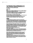
Suppose the LDR has a resistance of 500Ω, 0.5k Ω in bright light, and 200kΩ in the shade.
When the LDR is in the light, Vout will be:
One of the important factors which we should consider when constructing a potential divider is the resistance of the components. Let’s take the following example:
As we can see the Voutput hasn’t changed by much. This is because the resistance of the fixed resistor is so much larger than the LDR than any change in the resistance of the LDR only results in small changes in the Voutput. In order to get larger changes in the output we must make sure that components in potential dividers have roughly the same resistance.
Preliminary Experiment:
Carrying out a preliminary experiment can be very useful and this is why it was essential that I carried one. In the preliminary experiment I constructed a potentiometer which could be used to measure the rainfall over a given time.
Ogborn et al (2000) (CD Version), suggest that one way to monitor the level of liquid in a container is to use a float, which rises and falls with the level of liquid. Then the movement of the float needs to be converted into an electrical signal. One way to do this is to make the movement of the float turn the spindle of a rotary potentiometer.
This is precisely what I did in my experiment. I made a hole with the same diameter as the spindle in one end of the cardboard. I then used blu tack to secure the spindle stayed in the hole; this was necessary if the movement of the float was going to rotate the spindle. At the other end of the cardboard I used sealing tape to secure a copper wire to it. At the bottom of the copper wire I attached a polystyrene ball, which was going to act as the float. Below is a diagram of my experiment and how it was constructed:
During, my preliminary experiment I encountered problems. The most significant was the sensitivity of the device. The sensitivity of a measuring system is the ratio of change of output to change in input. The problem with my device was that the output voltage did not change for the first 150cm3 of water added into the beaker; however any addition of water after this caused a change in output given there was a change in input.
To manoeuvre this problem, I filled the beaker with 150cm3, and called this my starting point or 0cm3. Any additional water after this caused a change in the output voltage which was recorded. However, the results I obtained kept fluctuating, thus I couldn’t draw a calibration curve; therefore I was not able to analyse them correctly. This is why I chose to do my coursework on an LDR, as I couldn’t obtain more accurate results; making it easier to analyse the data.
Method:
To carry out my experiment I will need the following equipment:
Light Dependent Resistor (600Ω)
Variable Resistor (1kΩ)
Multimeter
Leads
Electrical Components Box
Power Pack
Light Bulb
Stopwatch
1 Meter Ruler
The sensor system I will be designing will be used for automatic night lights; therefore the LDR needs to be connected at the bottom of the potential divider. As I have explained in my science section (above), the voltage source (e.g. power supply) is divided in the ratio of the resistances. Thus, when it gets dark the resistance of the LDR increases meaning it gets a large portion of the voltage; as a result this high Voutput this turns the lights on.
This is a model of what my circuit will be like:
After connecting my circuit as above, I will go to a dark room and by using a 10V light bulb, I will try to obtain results as follows:
- Firstly, make sure that the LDR is in direct sight of the light bulb.
- Mark out 10cm points, starting from 10cm to 200cm.
-
Make sure the variable resistor is fixed at a resistance of 1kΩ.
- Place the bulb 10cm from the LDR (at your first point or mark).
-
Record the Voutput shown on your voltmeter and tabulate this.
- Repeat the last step for each different marked point up to 200cm.
- Tabulate the results and then draw graphs of them.
After drawing the graphs, I will be able to calibrate the Light Dependent Resistor. Once I have drawn my graph I should end up with a ‘calibration curve’. This is important for the sensor because a calibration curve tells you how to look up the input to a measurement system if you know its output.
Results and Graphs:
Using, the results above I will plot a line graph in order to calibrate my sensor. By doing this I can estimate the Voutput when the light bulb is placed 13cm from the graph of 155cm. On the other hand, I can also predict how far the light bulb needs to be from the Light Dependent Resistor, when the Voutput is 1.75 volts.
Calibration curves are very useful as we can find out the Voutput from a given distance of the light bulb and we can work out the distance of the light bulb from the LDR if we are given a Voutput. Below is a graph of the results above, as you can see this is a non-linear graphs are results do not increase with a constituent pattern or formula.
We can use our calibration curve above to estimate what the ‘Voutput’ will be when to ‘Distance (m) of the Light Bulb to LDR’ is 1.35. We can do this just purely from the graph without having to set up the experiment again.
To work out what the Voutput will be at a distance of 1.35 all we have to do is draw a vertical line upwards from 1.35m on the x-axis, until the line touches the curve. At that point where it touches the curve we draw a horizontal line towards the y-axis. At the point where this horizontal line meets the y-axis will be the Voutput we are looking for. This is shown below:
Analysis of Results:
The results above show what we expected; form our previous knowledge of LDR’s and potential dividers we know that the resistance of a LDR increases as the light intensity decreases. This is because the photons in the semiconductor do not have a high enough energy. Thus the electrons aren’t supplied with the energy needed for them to jump the conduction band and conduct electricity, thereby lowering resistance.
As a result, when the distance of the light bulb from the LDR increased, the light intensity decreased and this caused the resistance to increases. Furthermore, as we have set up our potential divider circuit with the LDR being on bottom and the voltage supplied to the circuit is divided in proportion to resistance, the Voutput increased in proportion to the resistance. We can see this from the graphs and the results.
The graph above shows that as the distance of the LDR to the light bulb increases for the first 0.90m the increase in Voutput is roughly proportional, in this first part of the graph. However, as the distance increases from this point (0.90m), the equal increments of length provide smaller changes in the Voutput than for the first part of the graph. This is due to the inverse square relationship of light which states that as the distance increases by 2 the light intensity decreases by ¼.
The increase in Voutput is bigger in the 1st part of the graph than for the same distance after 0.90m. This is because after this point the light intensity is so low that any further increase in distance virtually doesn’t change the light intensity by much therefore, the Voutput does not change by much. This causes the graph to curve after about 1.20m and as we can see above any further change in distance after about 1.80m hardly changes the Voutput. Therefore, we can make the assumption that if the x-axis (distance of light bulb to LDR) approaches infinity, 4.5 V on the y-axis is an asymptote.
The Inverse Square Law:
A source of light will look dimmer the further it is; this is because the energy flux spreads out and it’s less concentrated at a particular point.
The inverse-square law is ‘any physical law stating that some physical quantity is inversely proportional to the square of the distance from the source of that physical quantity’. This law applies to light intensity; as we increase the distance of the light source from a given object (LDR) or point, the light intensity decreases. The relationship can be shown by the formula:
where; I= light intensity & d= distance from object
This just means that if we double the distance, the light intensity decreases by ¼. This is because when the object is twice as far away, the area of the object becomes 4 times as big, therefore the energy needs to spread over four times the area; thus ¼ the light intensity. This relationship can best be understood by looking at a diagram, as below;
In this coursework I will use the inverse square law to find out whether my results are as accurate or not. However, because I could not measure the light intensity directly I will assign it with arbitrary units. The light intensity at a distance of 0.10m will be assigned the arbitrary unit of 1. If we now increase the distance by 10cm to 0.20m the light intensity should be 1/4 in arbitrary units according to the inverse square law. If we them triple the distance to 0.30m the light intensity will be 1/9 arbitrary units and so on.
In the aim of trying to prove that my results are correct and reliable, I will be drawing a graph of light intensity (in arbitrary units) against Voutput. If the curve is shaped liked a parabola and as the light intensity decreases the Voutput increases, then we will assume that our results are correct. From our previous knowledge and background research of this topic we know that as the light intensity decreases the voltage output increases, therefore this is what we are expecting our curve to show.
* Note: We have assigned the arbitrary unit of 1 to 0.10m; therefore all results will be based on this.
The graph shows that as the light intensity decrease, the Voutput increases; this is due to the resistance of the LDR increasing in dark light due to the fewer number of charge carriers, therefore the Voutput also increases. This graph shows that the two variables are inversely related, as one goes up the other goes down and vice versa.
Response Time:
Ogborn et al (2000), states that ‘The response time is the time a sensor takes to respond to a change in input. Changes which occur more rapidly than this will usually be averaged out. In any monitoring of a process, the response time of the measuring system must be short enough to detect important changes as they occur.’
Response time is very important component of a good sensor, street night lights need to respond in quick to any change in light levels (input), otherwise accidents might occur on the roads. Another situation where response time is particularly important is in greenhouses; plants need light in order to carry out photosynthesis, and make their food. One way to make them grow quicker is through artificial lightening; therefore a good response time means that during dark hours, the lights in the greenhouse will be turned on to enable the plants to photosynthesis.
As the above examples show, response time is particularly important in a sensor. This is one of the main reasons I chosen to investigate the time response of my LDR. To obtain the results for the response time, I set up my potential divider circuit in the dark room where I obtained my previous results for Voutput.
Subsequent to the setting up of the circuit I asked someone to assist me whilst I tried to obtain accurate results for respose time. Once, my circuit was set up correctly I asked someone to switch on the lights, whilst I used a stopwatch to time how long it took for the Voutput to change. The experiment was then repeated five times in order to obtain accurate results for response time. However, when carrying out this investigation, I recorded the time it took for the respose time to change back from dark to bright and vice versa to make sure the results were fair.
The table below shows the results I obtained from the 5 experiments I carried out; I have also worked out the mean time respose on the results.
The results above show that on average the LDR has a time response of about 1.32 seconds which is very quick. This would be ideal for nightlights or in a system which opens up and closes curtains when the light intensity changes outside.
This LDR might not be useful for camera shutter control. LDR can be used to control the shutter speed on a camera. The LDR would be used the measure the light intensity and the set the camera shutter speed to the appropriate level. Therefore the response time needed for a camera shutter would have to be much faster than the time response of my LDR.
Evaluation
As a whole I think this coursework went well as I meet my aim of constructing a potential divider circuit which could be used in either streetlamps or as a curtain opener/closure. I believe that the results I obtained where accurate to certain extend, however I do believe there were errors which might have slightly affected the results.
The method I used to carry out this experiment and obtain the results could have distorted the final accuracy of the data. One of the main problems, encountered when trying to obtain the results was fixing the light bulb at the same height as the LDR. This mean that as the light bulb was moved every 0.1m along the table its vertical positioning changed and was not always correctly in line with the LDR. This could have affected the results as the light wasn’t actually shining directly on the LDR. However, this was a systematic error and happened in each time the light bulb was displaced, therefore the results and the graphs drawn still represent the correct curve, although the curve might been higher than it should have been has this been controlled.
In addition, the experiment was only carried out once therefore the results might not be as accurate as those of someone who carried out the experiment three times and used the averages. Nevertheless, in order to make sure the results were accurate I plotted graph of the results as I recorded my results. Any result, which looked like an outlier on the graph, was repeated in order to check if it was a correct representation of the data.
Another way in which the results might have been skewed is due to measuring errors; this could have slightly affected the results. The ruler used to measure out the 0.1m gaps in the table was accurate to the nearest 1cm. This is a rather large error, however because it’s a systemic error it affects each result in the same way, therefore it shouldn’t make much of a difference to the final results. Furthermore, the voltmeter was only accurate to 2 decimal places; this again could have affected the results. The results obtained for the response time of could have been affected by measuring errors as well. The stopwatch was only correct to the nearest millisecond, and human error; time between the light was switched off and the time I started the stopwatch, could have distorted the results for response time.
If the experiment could be repeated, there would be a few things I would carry out differently in order to improve it. For example, I would try to repeat the experiment at least 3 times, and use the averages of these data as my results. This would give more accurate results. In addition, I would use a light meter to accurately measure the light intensity and plot this against the Voutput on the graph.
Apart, from the problems above I believe that the results are accurately as the experiment I was carried out correctly. By looking at the graphs and results we can see that there are no outliers so the general trend is correct.
Using my background knowledge of the science we have studied so far and carrying out my own research, I believe the results I obtained are still valid; regardless of the errors which undoubtly occurred.
Conclusion
As we can see form the graphs and results obtained, as distance of Light Bulb (m) to LDR increases the Voutput also increases. The graph shows that as distance increases for the first 0.90m the increase in Voutput is roughly proportional, for this part of the graph. However, as the distance increases from this point (0.90m), the equal increments of length provide smaller changes in the Voutput than for the first part of the graph. This is due to the inverse square relationship of light which states that as the distance increases by 2 the light intensity decreases by ¼.
As the distance increases further than 0.90m, any increase in the x-axis corresponds to a very small increases in the y-axis. This is because after this point the light intensity is so low that any further increase in distance virtually doesn’t change the light intensity by much therefore, the Voutput does not change by much. This is related to the inverse square law; at a certain distance the light intensity gets so low that any further increase in distance cause no further change in light intensity which cannot be detected by the LDR and thus Voutput wont change. This is what causes the graph to become non-linear and makes 4.5V on the y-axis an outlier. We can tell by looking at the graph that a further increase in distance from 2m will have no affect on the Voutput.
The reason for the increase in the Voutput is due to the increase in distance of the light bulb. As the light bulb is moved further away less light falls hits the LDR, meaning that there isn’t a high enough frequency absorbed by the semiconductive material inside the LDR, to give electrons enough energy to jump the band and lower the resistance. As results of this the opposite happens and the resistance increases as it gets darker. Relating this back to our previous knowledge of potential dividers; the potential is divided into the ratio of resistances, thus as the resistance of the LDR increases in dark light its ratio of the voltage increases.
As we can see form the graph, the results all follow a general trend, which causes the line of best fit to be a curve. This further reinstates that the results obtained are accurate and contain no outliers in the data.
In my hypothesis I assumed that as the light intensity increases the resistance of the LDR will decrease due to the extra number of charge carriers. In addition I noted that Voutput will depend on how the LDR is connected in the potential divider. If the LDR is to be connected on the top of the potential divider the Voutput will be high as the resistance of the LDR is low, whereas if its connected at the bottom of the potential divider its vice versa
The prediction was correct; I connected the LDR on bottom which meant that the Voutput increased as the light intensity decreased; this is due to the Vout receiving a larger ratio of the voltage supply.
In conclusion, the experiment went as planned and using my previous knowledge of potential dividers and light depending resistors in science I can assume that my results were accurate. Furthermore, the results matched my hypothesis and I can conclude despite there being errors the experiment went as planned and the results obtain were accurate.
Bibliography
-
Thompson C, Wakeling J (2003) AS Level Physics. Coordinate Group Publication.
-
Ogborn et al (2000) Advancing Physics AS. Institute of Physics
- http://www.doctronics.co.uk/ldr_sensors.htm (23 March 2008)
- http://www.technologystudent.com/elec1/ldr1.htm (25 March 2008)
- http://www.physics.iitm.ac.in/courses_files/courses/eleclab03_odd/light_dependent_resistor.htm (25 March 2008)
- http://www.reuk.co.uk/Light-Dependent-Resistor.htm (30 March 2008)