The following problem relates firm output decisions, market supply, and market equilibrium in a perfectly competitive market (further referred as PCM), that is, a market in which consumers and producers are price-takers.

ECON 2010-500, Fall 2003 Answer Key for Additional Exercise on Costs

Answer Key for Additional Exercise on Costs

Question 1. Complete the following table for a single firm in the short run.

Table 1. Cost accounting table for the firm. Letters in the brackets refer to logic used (see below). Answers are given in italic font.

Solution 1:

First we need to recall some relationships between various measures of cost accounting in the short run and definitions. We will number newly introduced formulas by bold numbers in brackets and then refer to them by number, for convenience.

We remember that (1). Definition for average total cost is (2) and for average variable cost — (3). If we divide both sides of equation (1) by quantity produced Q, and account for definitions (2) and (3) we get (4). Also, with definition (3), we can rewrite (1) as (5). Also, recall the marginal cost is defined as (6). Note, that we can also marginal cost as (7), since , because of the fact that (fixed cost does not change with quantity produced).

Logic (a). Remember, for each line we know quantity Q, shown in the first column. Also, for this table (only!) it is also true, that change in quantity ΔQ between two consecutive lines will be always ΔQ=1. Make sure you check this logic work when solving other problems, since increment in quantity could be arbitrary.

Logic (b). ATC if know TC is calculated directly using (2).

Logic (c). Note that for the first line (Q=0), the total cost TC consists just from the fixed cost FC (substitute Q=0 into (5)). Thus we can use FC=300 for the rest of the table analysis.

Logic (d). AVC by TC:. Here we show the equation number, to which we refer on each step of logic development, by small number in brackets under the “equal” sign. Note that we know TC and Q for this line, FC is always 300 (see Logic (c)).

Logic (e). MC by TC for this and previous quantity. Knowing TC for this and previous quantity produced, we immediately use equation (6), and the fact that ΔTCi=TCi-TCi-1 (8) for the i-th quantity. Specifically, for the second line: ..

Logic (f). TC by MC. We do exactly opposite to Logic (e). Knowing TC for previous quantity produced and MC for this quantity produced, we use equation (6) to find total cost for this quantity. Specifically, for the third line:

Logic (g). TC by AVC. We do exactly opposite to Logic (d). Knowing AVC for this quantity produced and remembering FC=300, we use equation (3) to find variable cost and then (1) to find total cost. for the line (4), where Q=3.

Logic (h). TC by ATC can be calculated directly from (2): TC=ATC*Q.

Question 2. Using the information in the table, fill in the supply schedule below for this individual firm under perfect competition, and indicate profit (positive or negative) at each output level.

Table 2. Decision making of individual firm

Solution 2:

We know that the quantity supplied is decided by ...

This is a preview of the whole essay

Logic (h). TC by ATC can be calculated directly from (2): TC=ATC*Q.

Question 2. Using the information in the table, fill in the supply schedule below for this individual firm under perfect competition, and indicate profit (positive or negative) at each output level.

Table 2. Decision making of individual firm

Solution 2:

We know that the quantity supplied is decided by the firm's manager, when he tries to maximize the total profit of his firm. Even before looking in the market prices report for today, he looks at the Table 1 on page , prepared for him by his cost accountants and performs some short-run analysis with respect to quantity-profit relation.

He knows that if he going to produce at all, he will fill in the column "Quantity supplied" directly from his marginal cost (MC) column in Table 1, because the rising part of MC(Q) curve is exactly his firm's supply S(Q) curve (, beyond the crossing of MC curve with the relevant average cost curve, see explanation in Appendix 1 on page ? if necessary) for the perfectly competitive market. Manager will choose quantity Q, which makes marginal cost of producing this Qth unit exactly equal to marginal revenue (which is price p for the perfectly competitive market).

Profit is just the direct difference between total cost of production and total revenue of selling Q units of output π = TR - TC, or, more exactly, π(Q) = TR(Q) - TC(Q). But total revenue is just TR(Q) = p*Q, since the price in the PCM does not depend from action of individual producers and the firm is able to sell all its output at price p regardless of production volume. On the other hand from equation (2) above we know TC(Q) = ATC(Q)*Q. So π(Q) = TR(Q) TC(Q) = p*Q ATC(Q)*Q = [p ATC(Q)]*Q (9). Thus the firm can get positive profit only if it produces at level of output Q, where ATC(Q) < p.

Will the firm ever produce at loss (where ATC(Q) > p, and thus π <0)? The answer is YES, in the short run firm may elect to produce in order to reduce at least part of losses associated with the fixed costs already irreversibly invested in business. So will firm produce no-matter-what as soon as it made some fixed investment? Here the answer is NO, because is does not make sense to produce anything if the money from selling next unit (MR, or price - when in PCM) do not cover the bare average cost of producing this same amount of units (AVC). Indeed, if our goal of production when π < 0 is reduction of losses then π = [p AVC(Q)]*Q - F (10) and looking how profit changes with each next unit produced, we see that , which is positive only when AVC(Q) < p. Thus manager can even before knowing the price in the marker rule out production at prices lower than that resulting from cross-section of MC and AVC curves.

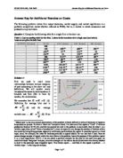
From Table 1 we see that MC first time overshoots AVC at Q = 4, where MC(4) = 80. Thus, unless price is at least $80, it is better for firm to just suffer loss of $300 fixed costs then incur additional loss on each unit on top of these $300… We will support this point below by more detailed analysis of case p = $60. Meanwhile we can put zeroes for "Quantity supplied" in lines for price $50 and $60. Apparently, profit from producing nothing (Q = 0) is just π = FC = $300, as we can see applying formula (10) above.

Table 3. Profitability analysis with p=$60

With the price equal to $60 situation is not much different from p=$50. Now MC(Q) = MR(Q) at Q=3. Nevertheless, although a small marginal profit is earned for second unit (see "Mprofit" marginal per-next-unit profit column in Table 3 above or same-name curve on "Unit Costs" graph to the right), the total profit for any number of units produced is still less than just fixed costs loss of -$300 (which is well seen from "Profit" column in Table 3 and also vaguely seen from the lowest dashed curve "Profit" on "Totals" graph).

This outcome is in perfect agreement with previous-page story, since the price = MR line on "Unit Costs" graph is clearly below any point of AVC(C) curve. So, at no output level the manager would be able to reduce loss from fixed costs. Thus, heavily-hearted, he orders to stop production before even starting it. He still may be fired for bad in-advance long-term planning, but in the short run he is making the right decision, preserving as much of the shareholders' money as he can at the moment. For p = $60 => Q = 0 and π = -$300.

Table 4. Profitability analysis with p=$110

From the Table 4 we see that loss reduction occurs from the first unit produced, because the revenue from it (equal to price or $110) exceeds the average cost of producing this first unit (which is $100). Now that the manager is sure to produce something he turns to the rule of profit maximization, which advises to select amount of output where MC(Q) = MR(Q) = p (the last equality holding only in PCM case). In Table 4 we can see that this rule actually works! Gray shaded cell in "marginal profit" column contains zero (MR MC = 0 => MR = MC) for Q = 5, the output volume which also maximizes total profit of the firm.

Minor confusion may arise from observing that two cells contain the same maximum profit value (for Q = 4 and Q = 5). But the look at the appropriately modified Table 5 below shows, that same profit in previous row is just a result of "discreteness" of table not being able to reflect the "continuity" of actual functions. In reality Q would be usually measured in thousands of units, so producing 4,500 units makes perfect sense. The smaller the step of the table, the closer the previous line to actually optimal line with MC=MR=p, becoming equal to it with the step in Q becoming sufficiently small.

Table 5. Effect of table "discreteness" explained

In fact this previous line with the same profit is inevitable by design when the price is exactly equal to one of the marginal cost values. The total profit changes by amount of Mπ= MR-MC= p-MC, which difference is equal to zero if we have table value of MC(Q)=p for some Q (Q=5 in our case here). Again this is result of "averaging" TC over ΔQ, whereas the "real" concave TC-curve reaches the slope MC(Q)=p only at the end of the segment ΔQ=[4;5] in our case…

If, as experiment, we will set the price slightly beyond the table value of MC, the ambiguity disappears even with the averaging of TC curve:

So, for p = $110 => Q = 5 and π = -$150. The firm is still making losses in the short run, but still operates at MC=MR to offset, at least partially, losses from the fixed costs.

Resulting Supply Curve is shown on the graph.

Question/Solution 3. Now suppose there are 100 firms in this market, all with identical cost schedules. Fill in the market quantity supplied at each price.

Suppose market quantity demanded is as follows.

Question/Solution 4. Fill in the blanks. From the market supply and demand schedules above, the equilibrium market price for this good is 180 and the equilibrium market quantity is 700 . Each individual firm will produce a quantity of 7 and earn a profit equal to 240 . (Hint: Market equilibrium happens where market quantity supplied equals market quantity demanded at the same price.)

Question 5. In 4 above, your answers characterize the short-run equilibrium in this market. Do they characterize the long-run equilibrium as well? If yes, explain why. If no, explain why not. (Hint: In a long-run equilibrium, no firm wants to enter or exit the market. This happens if firms in the market earn normal (zero) economic profits.)

Solution 5.

Apparently, the situation described in question/answer 4 cannot be a long-run equilibrium. Short-run equilibrium market price 180 [$/unit] had settled at level beyond the minimum ATC of individual firm (it is 140 [$/unit], from Table 1), which means that each firm earns economic profit (see formula (9) on page ). By the definition of the perfectly competitive market the entry in the market for new firms is easy, so they will tend to enter so to enjoy economic profits (non-existent in other, presumably in-long-equilibrium industries).

Entry of new firms will shift the supply curve out (to the right), which will lead to price decrease down to the level of the typical firm's minimum ATC. After that the long-run equilibrium will be reached.

Page of

“Short run” is the time-related characteristic of the problem at hand, defined in terms of character of inputs to the production process. We have a “short run” analysis at hand, if at least one of the inputs is “fixed”. If we have production function Q=F(L,K), and the time period we look in the problem is one month, then (a) labor L is a variable input (also called “factor of production”), since we typically can change the number of workers within the month by hiring/firing process, especially with hourly paid workers; (b) capital K would be typically a fixed input, since, for example, the lease for business premises is signed usually for not less than a year, thus we cannot change amount of capital within the time-frame in the problem, hence for purpose of this problem capital K is a fixed input/factor. NOTE: if we are asked to perform analysis for the year or two-year time-span, we would talk about “long run” analysis, since the manager will be able to decide (within that time frame) whether to enter in the premises lease altogether again. This makes capital — and thus all the inputs in problem — a variable input – in the long-run analysis.