Within the overall trends of bullish growth, and slow to negative growth in Japan, there have been significant fluctuations of GDP that have occurred over the last twenty years. In the early 1980s, the strong growth was mainly led by increases in consumption and the export of high technology products. Consumption was growing by 1.5 percent at the end of 1984 (Graph 3), and net exports had grown by 11.7 percent in the same year (Graph 4). The sharp growth of the GDP by 4.5 percent fell off the next year, as the increase in exports caused a heavy appreciation of the yen (Graph 7) creating a fall of exports by 3.5 percent in 1986. Consumption and (business-fixed) investment (Graph 2) also fell, taking the GDP with it. To offset this, the Bank of Japan (BOJ) loosened the already slack monetary policy, growing the money supply by 10.4 percent in 1986 and 11.2 percent in 1987 (Graph 5). A general IS-LM analysis in Figure 3 predicts that increase in the money supply will cause an outward shift of the LM curve from LM0 to LM1. This shift will lower interest rates to r1, which should therefore increase net exports of capital. The initial shift to LM1 will therefore be reinforced by the increase in NX and aggregate demand and GDP will increase further. Also, the falling interest rates will stimulate domestic investment and consumption which will contribute to the growth in GDP. The model predicts this quite well as in 1988 exports rose and GDP peaked at a 6.7 percent growth rate. Private consumption also increased by 2.4 percent and government spending by 6.2 percent (Graph 1). Interest rates (Discount Rates – Graph 6) actually increased from 2.5 percent in 1987 to 3.25 percent in 1988 and despite this Business Fixed Investment achieved impressive growth at 24.4 percent. The increased interest rates may have been a result of government spending (which shifts out the IS curve and raises interest rates) actually being greater than the increase in the money supply and so the model holds in this situation.
1990 was the pivoting point of Japan’s economy. A strict fiscal policy and a rise in interest rates decreased investment and lowered private consumption and consumer demand. GDP growth fell from 6 percent in 1990 to only 2.2 percent in 1991. At the root of this collapse, according to IS-LM analysis is the abrupt and extreme tightening of Japan’s monetary policy. The BOJ cut the money supply growth from 11.7 percent in 1989 to only 3.6 percent in 1990. Illustrated in Figure 4, this would cause an inward shift of the LM curve from LM0 to LM1 (cet. par). The result predicted is a decreased AD (from y1 to y0), and an increase in interest rates (from r0 to r1). Interest rates did in fact rise drastically to 6 percent in 1990 and investments fell -4.1 percent by 1991. The tight monetary policy continued, and consumption, exports and investment persistently fell until 1993. Japan was at a -1.0 percent growth rate in only three years!
From 1993 on, growth remained slow so the BOJ and the government employed less stringent monetary and fiscal policies in an attempt to drive the economy upwards. In 1994 the Bank of Japan cut interest rates from 2.5 percent to 1.75 percent – one of the lowest in its history, and public spending was boosted by 8.3 percent. As a result, investment was boosted from a -9.1 percent growth in 1993 to a positive growth of 4.1 percent by the end of 1994. The policies contributed to the economic recovery and with the accompanying increase in consumption and net exports that year, Japan’s GDP managed to climb out of negative growth to expand by 2.3 percent that year. The BOJ continued cutting interest rates to 0.5 percent in 1995 by loosening monetary policy and investment shot up 11.4 percent to help contribute to the boost of GDP to a local maximum growth of 3.6 percent in 1996. In 1997, “the government tightened its fiscal policy with a soaring tax rate to help pay its large debts from the previous years.” The increases in taxes reduced consumption as disposable income fell, which caused the fall in GDP growth to 0.6 percent in 1997 to -1.0 percent in 1998, despite the enormous increase in government expenditures that year.
Often policies take a while to kick in, and ‘trickle down’ to boost aggregate demand. This appears to be the case in 1999, as the increased government expenditures of 1998 seemed to be taking effect. Lenient monetary policies also continued to push down interest rates, stimulating domestic investment and consumption. By 2000, business investment had risen by 16.6 percent and private consumption was also on the rise. The yen also began to depreciate again, increasing net exports by 10 percent that year. All these factors helped raise GDP to a solid growth rate of 3 percent that year. Over the next two years, Japan’s GDP dropped with falling investment, government spending and exports, and rose the next year accompanied with the same variables. By the end of 2002, Japan’s GDP had grown slowly by 1.2 percent.
IS-LM analysis of the determination of GDP in Japan seems to fare well in this time period however it does have its short comings. For example, the interest rate chosen for the analysis was the nominal “Discount Rate”, which may not necessarily be relevant to the analysis. There are other interest rates such as the “Prime Lending Rates”, which may be more useful. Also, interest rates and consumption in Japan did not seem to respond strongly to monetary policy in the 1990’s as IS-LM predicts. An explanation may be that Japan was in a liquidity trap (see Figure 5), where outward shifts in the LM curve will have no effect on either interest rates or aggregate demand. Keynesian economists argue that a Liquidity Trap would arise if “market participants believed that interest rates had bottomed out at a “critical” interest rate level and that rates should subsequently rise, leading to capital losses on bond holdings.” This was quite possible in Japan at that time as discount rates had reached a low of 0.5 percent. However, in the presence of a liquidity trap, the interest rate elasticity of money demand is predicted to increase as the interest rates fall to zero but a study by Isabelle Weberpals found it to actually decrease as interest rates fell. If Japan was not in a liquidity trap at this time, then the IS-LM model proves to be quite inaccurate. Another problem with using this model is the set of assumptions it relies on: that investment is a function of the interest rate alone, consumption is a function of disposable income alone and money demand is a function of both the interest rate and income. These assumptions truly do not hold in real world economies as consumption, investment and money demand are all subject to such variables as personal preferences and speculation as well. It is necessary therefore to look at another model in order to complement or test the validity of the IS-LM analysis of Japan’s GDP growth.
In Neoclassical Growth Theory, for a given year, GDP (Y) depends on the output per worker (y) and on the labour force (L):
Y = y.L (3)
Y” = y” + L” (3.1)
This model asserts that output per worker depends on the capital per worker, therefore output (Y) is a function of the capital stock (K) and the labour force (L).
Y = F(K,L) (4)
In the simplest model of a closed economy that does not have a government sector, which is obviously not the case in Japan, the capital stock (K) changes by the amount of real investment (I). In this type of economy, in equilibrium the change in capital stock per period (K’) must equal saving (S):
K’ = I = S (5)
Ignoring the other complications of its derivation, A Solow Diagram that assumes steady state (where the capital/labour ratio does not change) looks like this:
In Figure 6, σf(k) measures the availability of new capital per worker (where σ is the marginal propensity to save), or saving per capita and nK measures the (per-capita) capital requirements of the new workers. Steady state (SS), where σf(k) = nK, occurs at k* where k is the capital per worker (K/L). Measurement is in units of output. A decrease in the saving rate reduces investment, and the pre-SS growth rate in the transition to the new steady state and the steady state itself. In steady state, the growth rate of output per capita (y”) is zero, and since y”=Y” – L”, in the steady state
Y*” = L” = n. Therefore, the steady state values of Y and K grow at the labour force growth rate. The lower the labour force growth rate, the lower the growth rate of output and capital in the steady state.
The labour force is defined as the number of workers who want a job at the existing wage rate. Figure 7 shows the growth of Japan’s labour force and the growth of Japan’s GDP for the last twenty years up to 2002. “When it comes to the ageing of the population, Japan is further down the road than any other developed country.” Japan’s recent low fertility rate has been compounded by its significant rejection of immigration. As a result, in 1991 Japan’s labour force growth rate began to decrease drastically, which proved to have a strong effect on the growth of Japan’s GDP.
Figure 8 shows the saving rate per year and the growth of Japan’s GDP for the last twenty years. The saving rate began to fall drastically in 1991, just around the same time as the fall in the growth of the labour force. Before 1991, Japan was known for its excessive savings rate however a number of factors caused it to drop that year. “First, savers at both the individual and corporate level are getting skimpy returns on their investments owing to near-zero interest rate levels. Second, the savings rate is being hit by rising unemployment and declining incomes across the board. Most importantly, older Japanese are being forced to spend down their savings faster than they anticipated to support unemployed or poorly paid offspring.” In the same year, Japan entered its “Heisei Recession” and GDP growth slowed drastically.
The saving rate has only dropped even more since that time, and fell to 0.06 percent at the end of 2002. In part the fall in savings was due to the fall of GDP itself, but the continued decline has created problems in recovering growth and also compounded the initial fall. The Solow Model provides an analysis on why the combined fall in the growth of the labour force and the fall in savings rates were causes of the subsequent sluggish growth of Japan’s economy.
Figure 9 is a Solow model showing the effect of the fall of both the saving rate and the growth rate of Japan’s labour force on the growth rate of Japan’s real GDP in 1991. The model begins at steady state at k*0 for simplicity’s sake but this may well be an unrealistic assumption for Japan at this time. The decrease in the saving rate shifts the σf(k) curve down from σ0f(k) to σ1f(k). The decrease in the labour force growth rate lowers the nk curve from n0k to n1k. A new steady state is established at k*1, at the intercept of n1k and σ1k. Since the capital per worker has increased to k*1, the output per worker will be higher. “However, the fundamental growth equation implies that the growth rate of output per worker in one steady state, as in the old one, will be zero, so that the growth rate of output per worker does not change from one steady state to a new one.”
However, output will fall in the transition from k*0 to k*1. This may have been the cause of the fall in Japan’s GDP growth in the early 1990’s. The Solow model predicts that in steady state, countries with lower labour force growth rates and lower savings rates will have the same (zero) growth rate of output per worker, but a lower growth rate of output. The model suits the data quite well, as Japan’s saving rate and labour force growth rate were both high in the 1980’s, along with the growth rate of its GDP, and were both lower in the 1990’s when Japan entered its recession. On the other hand, the theory does have its flaws. Perhaps its worst assumption when considering Japan’s economy is that it is closed. Japan is highly dependent on both imports and exports of financial capital, raw materials, and finished products. Also, the extremely low interest rates have caused Japanese corporations to invest heavily in foreign countries to receive hopefully higher returns. This, along with the fall in saving rates has hindered Japan’s ability to build up capital and therefore speed up growth. The presentation of the Solow model in this case has not adjusted for influences from outside economies and must do so in order to properly analyze growth in Japan.
In general, the fluctuations in Japan’s GDP were explained quite well by both growth theory and IS-LM analysis. The models however are too simplistic and need adjustments for the structural aspects of Japan (especially its susceptibility to influences of outside economies. This paper also failed to incorporate models of expectation such as the Friedman or Lucas supply rules which are just important as the IS-LM and Solow growth models in analyzing the output growth of an economy. They therefore must be examined for a proper study. Today, Japan is still feeling the effects of the collapse of what has come to be called as the “bubble economy” in 1991, and is still growing at a sluggish rate.
Bibliography
AsianInfo . “Japan’s Economy.” 2000
< http://www.asianinfo.org/asianinfo/japan/pro-economy.htm>
The Bank of Japan. “Bank of Japan Statistics.” 2004
< http://www.boj.or.jp/en/stat/sk/data/skeall.pdf>
Boschini, Anne. “Growth Theory 1.” Jan 2004
<http://people.su.se/~bosch/lect1.pdf>
Bremner, Brian. Business Week Online. “Japan’s Dangerous Savings Drought.” 9 June 2003
< http://www.businessweek.com/magazine/content/03_23/b3836159_mz035.htm>
Gittins, Ross. F2 Network . “Japan will Never Return to Decent Growth.” 2002
< http://www.smh.com.au/articles/2002/10/27/1035683304208.html>
Handa, Jagdish. Macroeconomics. Montreal: Mcgill University, 2003-2004
Johnsson, Richard. The Ludwig von Mises Ins. “The Liquidity Trap Myth.” 19 May 2003
URL: http://www.mises.org/fullstory.asp?control=1226
Krugman, Paul. “Japan’s Trap.” Oct. 2003
<http://www.pkarchive.org/japan/japtrap.html>
Kuichi, Yoshiba; Akifumi Nakao and Takashi Baba. “Macroeconomic Analysis of the Monetary Policy in Japan.” Jan. 2001
< http://www-personal.umich.edu/~kathrynd/japan.556.pdf>
Powell, Benjamin. The Ludwig von Mises Ins. “Explaining Japan’s Recession.” 3 Dec. 2002
< http://www.mises.org/fullstory.asp?control=1099.
Putturman, Lucas. Ch. 2: Economic Growth: Theory and Empirical Patterns. Topics in Economic Development. New York: W W Norton and Company, 2001
< http://www2.montana.edu/jantle/pdf_files/econ317/Perkins2sec1.pdf>
Shinotsuka, Eina. The Bank of Japan.“Japan’s Economy and the Role of the Bank of Japan.” 27 May 2000 <http://www.boj.or.jp/en/press/00/ko0007b.htm>
Ueno, Daisaku. “Downtrend in Japan’s Economic Growth.” Accessed: 6 Feb. 2004
<http://www.iptp.go.jp/reserch_e/monthly/m-serch/finance/1997/no104_2/UENO.html>
Weberpals, Isabelle. The Bank of Canada. “The Liquidity Trap: Evidence from Japan” 1997 <http://www.bank-banque-canada.ca/publications/working.papers/1997/wp97-4.pdf
Appendix A: Graphs of Relevant Data
Appendix B: Data Tables
Handa, Jagdish. Macroeconomics “Ch 14: Flexible Exchange Rates”
Handa, Jagdish. Macroeconomics. “Ch. 4: IS-LM Analysis” pg 62
Ibid, “Ch 14: Flexible Exchange Rates”
Anonymous, Japan’s Economy
Eiko Shinotsuka, “Japan’s Economy and the Role of the Bank of Japan”
Weberpals, Isabelle. “The Liquidity Trap: Evidence from Japan” pg 9
Handa, Jagdish Macroeconomics “Ch. 16: Classical Growth Theory”
Putturman, Lucas, “Economic Growth: Theory and Empirical Patterns” pg 12
Handa, Jagdish Macroeconomics “Ch. 16: Classical Growth Theory” pg 14
Gittins, Ross “Japan will Never Return to Decent Growth”
Bremner, Brian “Japan’s Dangerous Saving Drought”
All Data From: The Bank of Japan Website. “The Bank of Japan Statistics”