Vacuum Chamber Investigation
Planning:
Apparatus List:
When conducting the experiment I will need the following pieces of apparatus:
* Rotary Vacuum Pump
* Vacuum Chamber
* Manometer
* Valve
* Short Pipe
* Long, thin pipe
* Stop Clock
Apparatus Diagram:
Safety Considerations:
It is important that when setting up and carrying out the experiment no objects are poked into the belt drive mechanism of the rotary pump. The mains voltage in the mains powered equipment is also dangerous but is screened in normal use. Obeying these two safety points will help prevent physical injury and electric shock.
Variables which could affect the Experiment:
* The length and diameter of the pipe connecting the vacuum chamber to the vacuum pump.
* The size of the vacuum chamber.
* Changes in atmospheric pressure may affect the experiment. This is perhaps one of the more major variables because it can account for up to plus or minus 50 mbar.
* The consistency of the Rotary Pump may be a major variable in this experiment. It is unlikely that its performance will remain constant when evacuating the vacuum chamber. This is because of heat build up in both electrical and mechanical components such as the mains transformer and seals when pumping takes place.
* Changes in room temperature may cause variable characteristics in the experiment. Changes in temperature may affect several items such as the efficiency of the rotary pump and the viscosity of the air travelling through the system.
* Due to the nature of the apparatus set-up there are a number places where air may escape. These are mainly where valves and couplings are located, such as the air inlet valve, the main valve and couplings to the pipe, manometer, vacuum chamber and vacuum pump.
Variables that will be varied:
* The length and diameter of the pipe connecting the vacuum chamber to the rotary vacuum pump will be varied. In this experiment two different pipes will be used. The first one will be a short, wide pipe (10cm long, 3cm diameter). The second will be a much longer pipe (10m) and be considerably narrower in diameter (4.8mm).
Variables that will be kept Constant:
* The initial pressure in the vacuum chamber will be kept constant in this experiment. The pressure will be brought up to atmospheric pressure (approximately 1000 mbar) for both the short and long pipe experiments.
* The size of the vacuum chamber will be kept constant.
Method:
The apparatus will be set up as illustrated in the apparatus diagram with the short, wide diameter pipe connected. At this stage the vacuum chamber will be evacuated in order to note and take into consideration systematic error. The chamber will be evacuated by simply closing the air inlet (admittance) valve, opening the valve to the pump and finally starting the pump. When the manometer reads approximately 2 mbar, the evacuation has finished. It is now necessary to know more accurately what the exact pressure is in the chamber even though it is evacuated. I will now change the manometer into the low pressure scale (less than or equal to 200 mbar) and note the pressure reading. This is the systematic error and I will now have to correct every reading I take to allow for this zero offset.
Once the zero offset is established the vacuum chamber will have to be taken back up to atmospheric pressure (approximately 1000 mbar). To do this I will close the valve to the pump and open the air inlet (admittance) valve. Again, once the manometer is reading a constant value close to 1000 mbar (on the standard pressure scale) the chamber is ready to be evacuated. I will now close the air inlet (admittance) valve, start the clock and open the valve to the rotary pump. I plan to measure the pressure at 20 second intervals until the pressure ...
This is a preview of the whole essay
Once the zero offset is established the vacuum chamber will have to be taken back up to atmospheric pressure (approximately 1000 mbar). To do this I will close the valve to the pump and open the air inlet (admittance) valve. Again, once the manometer is reading a constant value close to 1000 mbar (on the standard pressure scale) the chamber is ready to be evacuated. I will now close the air inlet (admittance) valve, start the clock and open the valve to the rotary pump. I plan to measure the pressure at 20 second intervals until the pressure reduces to approximately 2 mbar. I will repeat this procedure in order to take average values of pressure at the 20 second intervals.
For part II of the experiment it will be necessary to carry out the above procedures again, except this time using a long, narrow diameter pipe. To connect the new pipe: I will first of all close the valve to the pump and use the air admittance valve to let the pressure in the container up to atmospheric pressure. I will now close the air admittance valve and disconnect the coupling between the valve to the pump and the container. The long, narrow diameter copper tubing can now be connected between these two couplings. Once the pipe is connected I will open the valve to the pump and measure the pressure every 20 seconds, as before, until the manometer reads approximately 5 mbar.
Modified Apparatus & Selected Instruments:
Due to the fact that the long, narrow pipe is 10m in length it will be necessary to 'coil' this pipe in order to fit the apparatus set up in the laboratory. It is important that no 'kinks' are created when coiling the pipe otherwise the flow of air will be severely impeded.
There are only two measuring instruments in this particular investigation. The first is a stop clock to measure time intervals between pressure readings and overall evacuation time. The second instrument is a manometer. This device will be connected to the vacuum chamber and will be used to measure pressure.
Sensitivity & Accuracy of Measuring Instruments:
Both the stop clock and the manometer are accurate and sensitive digital instruments. In terms of measuring time, measuring to the nearest second is perfectly adequate in this experiment. Therefore the digital stop clock is more than accurate enough.
Due to the fact that I will be dealing with pressures at and below atmospheric pressure it will be more convenient to work in the units millibars. In these units atmospheric pressure is 1 Bar, i.e. 1000 mbar. (We know, of course that the actual atmospheric pressure depends on the weather at a given time. Typically, meteorological variations of 'atmospheric pressure' are approximately plus or minus 50 mbar). A manometer is the perfect instrument to carry out this kind of measurement as it displays pressure in millibar units. It also has the ability to work in the low pressure scale (less than or equal to 200 mbar with a 0.1 mbar resolution. This particular feature will come in useful when determining the zero offset. However when measuring pressure for evacuation purposes, measuring to the nearest mbar is ample.
Treatment of Results:
Graphical plotting will be used to extract information. Results for the first part of the experiment will be plotted graphically. Pressure (mbar) against Time (s) will be plotted and also further logarithmic graphs. The results for the second part will be treated in a similar fashion but with more analysis due to the more complex nature of air flow through the long, narrow pipe.
Pilot Experiment:
As stated earlier in the project, it will be necessary to carry out an appropriate pilot experiment. This will put the investigation into a more concise context. It also aids planning.
I plan to carry out a routine experiment that in some way simulates the actual pumping speed experiment. The pilot experiment will involve discharging a known capacitor through an unknown resistor. The aim here to find the value of the resistor. This will be achieved through graphical plotting (Voltage against Time) and capacitor formulae. The Voltage against Time graph will also be plotted logarithmically in order to understand how the capacitor discharges. Through finding the value of the unknown resistor, this will emulate the pumping speed experiment when I will try to find out the speed of the pump.
The second part of the pilot experiment is to test a much larger resistor of known resistance. The objective here is to see how a larger resistance affects the discharging of a known capacitor. In both parts of the pilot experiment a 100 micro Farad Capacitor will be used. This second part to the pilot will hopefully emulate the effects of the long, narrow pipe in the pumping experiment.
Safety Considerations for Pilot Experiment:
This is a relatively safe experiment. However I must take care not to get an electric shock from the charged capacitor.
Apparatus List for Pilot Experiment:
* 100 micro Farad Capacitor
* Resistor of unknown resistance
* Resistor of known resistance (this will be selected after the value of unknown resistor is found. The selected resistor must be of a much larger resistance)
* Voltmeter
* Stop Clock
* Power Supply Unit
* Connecting Wires
Circuit Diagram for Pilot Experiment:
Analysis of Results from Pilot Experiment:
From the graph of average potential difference (Volts) against time (s) the value of the resistor used to discharge the 100 micro Farad Capacitor may be calculated.
We know that the capacitor discharge curve (P.D against Time) can be modeled by the following equation that is derived using calculus:
Q = Q0 e
Here Q0 is the charge stored when t=0, and e is the number known as the exponential number. This exponential number, e is approximately equal to 2.718. The above equation can be re-modeled in order to tell us how the voltage changes. Substituting the equation Q = CV (where C is the capacitance of the capacitor, and V is the potential difference or voltage across it). Canceling C, we get:
V = V0 e
After a time equal to RC the voltage across the capacitor will drop to 0.37 or 37% of its original value. 0.37 or 37% is derived from the reciprocal of the exponential number, e. Where 1/e is approximately equal to 0.37 (or 37%). From this we can deduce the following formula, which is known as the time constant of the discharge. This time constant is used as a measure of how fast the resistor-capacitor combination discharges. It is sometimes represented by the Greek letter ? 'tau'. Where :
? = RC
From the above set of derived formulae I am now able to calculate the size of the resistor used in the discharge of the 100 micro Farad capacitor.
From the graph of Average P.D against Time, it takes 15 seconds for the voltage to drop to 37% (1/e) of its original value of 4.8V. Therefore, from the time constant formula we can calculate the resistor size:
? = RC
15 = R x 100x10
R = 15/100x10
==> R = 15K?
Therefore the size of the unknown resistor used to discharge the 100 micro Farad Capacitor in part one of the pilot experiment is 150,000? or more simply 150K?.
As well as this result we can see that from the graph of ln (natural log or log to the base e) Voltage against Time, a strait line forms. This clarifies that the capacitor did indeed discharge exponentially. This is what one would expect by virtue of the equation that describes the discharge. We know that an exponential equation, lets say in the basic form of y = k x can be rewritten by taking logs to the base e of both sides in order to turn it into an equation in the form y = mx + c. Take the following example:
y = k x
where k and x are constants
Taking logs of both sides of the equation:
ln y = ln k x
ln y = ln k + ln x
ln y = ln k + n ln x
==> y = c + xm
Thus, by plotting ln y against n a straight line will form, of gradient ln x and y intercept
ln k .
Through this pilot experiment this has now been proved.
Now that part one of the pilot experiment is completed and the value of the unknown resistor is known, comparisons can now be made with discharges through larger resistors. For part two of this experiment I selected a 700K? resistor for the 100 micro Farad capacitor to discharge through. Again a graph of Average P.D (Volts) against Time (s) was plotted as well as a logarithmic graph to confirm that the capacitor discharged exponentially.
Analysis of Part II of Pilot Experiment:
Quite clearly the larger resistor made the overall discharge time much longer. This is not surprising because of the fact that the time constant equation gives us a measure of how fast the resistor-capacitor combination discharges. The capacitor used in this part of the experiment was the same as the one used in the first part (100 micro Farad). However the resistor was much larger. A 700K? resistor was used in place of the 150K? resistor. Therefore the time constant was much larger, and hence the capacitor took longer to discharge. By comparing the values of the time constants in the two parts of the experiment we can see that the 700K? resistor made the overall discharge time approximately 4.5 times longer than with the 150K? resistor:
Time Constant of Pilot Experiment I: 15 seconds
Time Constant of Pilot Experiment II: 75 seconds
==> 70/15 = 4.67
However it did discharge in the same fashion: -exponentially. This was again confirmed by the logarithmic graph. This factor is important, because it tells us that regardless of the resistor size, the capacitor will still discharge exponentially.
From the pilot experiment I have improved my understanding of exponentiality. This will prove to be important in the actual experiment; however I do not feel that my plan needs any revisions at this stage.