Porosity
Multipliers are assigned on a well-by-well basis to increase or decrease porosity. An option is to renormalize. In this case pore volume is increased along streamlines connected to certain producers, but the overall pore volume is preserved by renormalization.
Application of AHM using Streamlines
In SPE paper 747121, three examples of the application of AHM using streamlines are discussed. Within the three example cases there is one case where a finite difference model is considered. The results of each of the examples are given with brief discussions; stating whether or not the technique was successful and ranking them in terms of most successful/efficient. All examples are real life cases, which have different results to the synthetic cases.
AHM Technique: A Streamline Model
The initial simulation for this model showed early water break-through for most of the wells accompanied by an insufficient productivity. Also, on a field wide basis, the overall water production was over predicted by a significant margin during the early life of the reservoir. When AHM was applied to this model, changes were made to this permeability, porosity and the heterogeneity of the model.
Figure 01 – Field-wide water-cut performance for Model. White is
History, orange is the final history-matched model, and red represents the initial model results1
To increase well productivity, the horizontal permeability had to be increased. First a reduction in Kv was made to increase the model stratification and then to stabilise influx and match delayed water break-through, Kv was increased.
The changes in permeability heterogeneity were done through a DP renormalization. The increase in heterogeneity meant early water break-through of the displacing phase and more dispersed fractional flow.
The results show that using this method a satisfactory match is achieved for this particular reservoir (full reservoir description available in SPE 747121). The match was achieved by changing the DP coefficient for all the wells; by changing the pore volume of roughly half of the wells and applying Kv and Kh multipliers to approximately 20% if wells. The changes that took place were quite modest; averages of 20%, but some were much higher as the mismatch between historical and model data was greater.
A Finite Difference Model
In this example there was no use of streamlines. It used grid block modelling. Before AHM was applied, simple increases in the size of the surrounding aquifer resulted in an inadequate match. This also caused a discrepancy in the model and field pressure decline, especially at late times.
Even though a good match was achieved, a significant number of shale regions exist in the reservoir that limits the vertical connectivity of the field. The lowering of Kv/Kh ratio of individual grid blocks was consistent but time consuming.
The reason behind my mentioning of the finite difference case is to show that even with the aid of AHM, working on a grid block model can achieve a relatively good match, but compared to the use of streamlines, this method is deemed very slow, hence, time consuming.
Two examples of the application of AHM on finite difference models are discussed in SPE paper 490002. The first example it can be seen that decreasing the ‘Dykstra – Parson’ coefficient (DP), results in a more homogeneous distribution of permeability resulting in later breakthrough of injected water, and vice versa. This was applied to some of the wells in the example. A third of the wells had undergone an increase in the DP coefficient resulting in earlier breakthrough, which was observed in the reservoir.
When AHM was applied, it took 6 iterations to achieve a reasonable match. A small improvement is observed by the match obtained through AHM, although it wasn’t significant. The only significance was that the 6 iterations took a week to compute, compared to the 2 months required by traditional methods. The methods of AHM application in SPE paper 490002 took longer as this was an earlier paper than reference 1.
In the second example2, a full field model of the reservoir was developed using geo-statistical software. Prior to history matching, water production in the model is considerably less than the observed in the field. Simple increases in the size of the surrounding aquifer are inadequate to match the observed water production and cause a discrepancy between model and field pressure decline, especially during late times.
When AHM was applied, a well-by-well analysis of the field was conducted, which lead to the changes of three principle variables: Horizontal permeability, Kv/Kh ratio and the local pore volume. Lowering of the Kv/Kh ratio of the grid blocks is consistent with the aspect of reservoir geology. Decreasing the ratio led to a greater horizontal encroachment of water. A renormalisation of the pore volume was also made. This re-distributed some of the volume as indicated by the production data of this field (see paper 490002).
The results show that an excellent match is obtained after less than a dozen iterations, which took place within a week. It is also stated that for this particular example, three models were built; each to address a different objective. One of the models contained 25,000 grid blocks; another 100,000; and lastly 250,000 grid blocks. The models were matched sequentially with increasing size. The results showed that the parameters used for the 25,000 grid blocks were identical to that of the 250,000.
For most geological consistent models, this result can be achieved, however, in practice it mat not be the case.
History matching in a well-by-well basis using AHM proved very satisfactory; matches were obtained with a few iterations. The next section discusses the application of AHM on to an Arabian field, and also further developments of AHM.
The Saladin Reservoir: A Finite Difference & Streamline Model1
Initially a Finite Difference model was used for history matching, the results obtained from the simulation were satisfactory but run times were typically 10 – 15 hours. In an attempt to reduce run times, the model was coarsened; this involved reducing the number of cells that made up the model. Run times were reduced to 5 – 7 hours; however, the history match was significantly different and unsatisfactory.
To further reduce run times whilst retaining fine scale, a streamline model was chosen instead. This method reduced run times to 2 hours and the streamline model was easily constructed.
For this example, the application of streamlines was immensely beneficial. The filed had pore volume multipliers applied to account for the full extent and aquifer support. Sizing of the aquifer to the Northeast and Southwest of the model was crucial to matching of individual wells (see paper1 for figure).
The 3DSL model was used in the understanding the effect of the aquifer on the drainage areas and well patterns. The simulator was then used to predict the oil rates.
In terms of history matching, using conventional history matching parameters assisted by streamlines, most of the wells for the Saladin reservoir were matched, except two. Well mismatch problem was overcome by continuing matching process using AHM. For this continuation, a streamline pattern representative of flow for the whole reservoir was chosen. Improvements to particular wells were performed by changing the DP coefficients and pore volume. In this way, the heterogeneity around a well could be modified to improve well match. The field history match achieved was very good, see figure 03.
Figure 02 - Streamline display showing individual Figure 03 - Saladin reservoir-field history
wells and their Drainage areas1 match1
Summary of the Technique
The AHM technique uses unique information contained within the streamlines to assist the traditional method of history matching.
The first case discussed in the paper shows the utility of a heterogeneity renormalisation technique coupled with streamlines to affect a well-by-well history match. The second case, changes to Kv/Kh ratio can be quickly applied to achieve desired results. Although with the second method, alterations needed for individual grid blocks was very time consuming. Reducing the layering of the model did result in reducing time of simulation, but the match achieved was not as desired. The last case shows the extent of the usage of the finite difference model and how quickly streamlines with the aid of AHM, match can be achieved.
In all three examples, the changes that were made were within general uncertainty of the initial data. This is the advantage of AHM: relatively modest changes are required to obtain a history match from a well constructed geological model.