Explanation of how these inputs are calculated:
Each new user start with a value of £200.00.
Depending on age and other factors this
Value of £200.00 is multiplied.
Each section the value is multiplied by the
Multiplier figure and all added together.
Example:
Age 17-19= 200*4.4
+
Sex-male= 200*1.2
+
Area-med= 200*1.5
+
No claims 1yr= 0.20*200
+
Type third party= 0.39*200
= £880+£240+£300+£40+£78= £1538.00
Processing requirements:
•Have a separate sheet of car details showing IG numbers
•Have a separate sheet of multiplying factors
•Have a quotations sheet where the quote is calculated by using formulas.
(Information is taken from the cars and multipliers sheets to work out the quote)
•Formula multiplies the basic cost of the car with all the multipliers to get the cost of the quote.
•Produce a final quotation price by multiplying the figure with the no claims percentage.
•Add VAT onto the final cost. (0.175*...)
Output requirements:
•Full quote details on screen and details are provided on multiply outputs.
•Fully customised and professionally printed output with company logo and header.
•The output will include all the personal details of the user.
•The output will include which policy the user has selected.
•The output will also include the make/model and specification of the end users car.
•The output will include a price including VAT on the basis of their personal details, their policy details and on their type of vehicle.
The Macros Iam going to use in my system are:
•Iam going to make a macro to automate the filling of the quotes into the customer
This macro will fill away the end users quotes; into a separate worksheet.
This macro takes along time to record as it involves copying each of the necessary cells form the quotes sheet, then pasting the cells onto the customer’s worksheet.
I will do this by selecting the first black row on the customer’s worksheet, clicking insert, rows. I will produce the macro so every time a new quote is saved, it will be
added in at the top, without replacing old quotes.
• Also Iam going to use a print quote macro; this will allow the user to print their quote at the touch of a button. I did this by: stat recording macro, d to the worksheet, from menu clicked file, print, O.k. and finally switch back to the Quotes worksheet and stop recording.
•Also Iam going to add an Auto-open macro and an Auto close macro.
Iam going to set up an auto-open macro that would remove the gridlines, sheet tabs, row and column headings and scroll bars, when the system opened.
I will set this macro by start recording, clicking tools, then Options, uncheck the gridlines, sheet tabs, scroll bars and row column headers. Uncheck the formula bar and status bar. Clicking view, toolbar and remove the Standard and formatting toolbar; then Stop recording.
User requirements:
To get an insite into what the dealer expected from my system I wrote the manger Bill Walker a letter asking him: “Please can you list the user requirements you want me to do when producing the insurance quote system for your dealers.
Several days after, Bill replied with this letter below:
Objectives:
•The system will have a section for the customer details, which is well set out. It will be easy and quick to fill in details.
•The system will have a section for the car details, which will be well set out. It will be quick and easy to fill in the details.
•The system will have a section with all the multiplying factors clearly stated, and will be easy to amend if needed.
•The system will have a final Quotation page; this will take into account all the information like car details... Which will be calculated using formulas, and formulated to give a clear and professional Quote.
•The system will be able to store customer details separately for future reference.
•The system will use formulas which will be the most advanced formulas to give quick and accurately calculated quote.
•The system will use validation rules. This will prevent the number of mistakes occurring for the end user.
•The system will use macros to navigate around the system quickly and efficiently.
•The system interface will look professional, to devise this I will use drop down menu’s and pointers and spinners on the sheet.
•The system must printout a quotation sheet, in consideration to A4 user’s printers. The output will be landscape.
•The colour scheme will be basic yet professional looking.
•The text colour will also be smartly addressed to each worksheet; with red font on
The final output, which matches the red Vauxhall Logo.
•The font of the text wills all be New Times Roman; but size may vary between worksheets.
•The system will be able to add VAT onto the final price to give a Total Cost.
• VAT is 17.5 % multiplied by the total cost to give a final cost.
Implementation:
First I had to open Microsoft Excel. To do this I clicked on START and then highlighted Excel and left clicked to OPEN it.
Or alternatively you can click ‘Start’ then ‘All Programs’ and then ‘Core Programs’ where Excel will be located.
Setting up the Insurance Groups worksheet:
I started off by setting up a sheet that would contain all the information of on the cars and their insurance groups. First of all I entered the number per car in column A; this is so later, the cars can be looked up easily. I entered the makes of the cars in column B, the model of the car in column C, the IG of the cars in column D. The Insurance Groups number from 1 to group 20; this range will easily include the Vauxhall cars Insurance Groups. I entered the basic premiums in column I.
I also added a column in E that would produce a unique name for a car by combining the make and model. I did this by typing in a formula that combined the contents of column B and C.
I then highlighted the area A1 to E10 and went to ‘Insert’, ‘Name’ and then ‘Define’. I called this area ‘Groups’. I also highlighted from H1 to I12 and named it ‘Costs’.
Setting up the Multipliers worksheet
The second sheet I set up was the multipliers sheet, which would hold all the factors and their multiplying figure.
I entered the separate multipliers onto the sheet, age, sex, area, no-claims bonus and the type of insurance.
I entered numbers in column A, which will be needed later to lookup the multipliers. In column B I entered the different multipliers and in column C, I entered the multiplier figure.
The figure is the multiplier which is used in a special formula to give the overall cost. For example, for a Male driver it is x1.2, whilst for a Female driver the multiplier is x1.0.
Setting up the input controls onto the quotes worksheet.
This is the major worksheet of the system, and takes information from the groups and multipliers sheets and works out the quotation.
I entered the labels for the customer’s title, forename, surname, address, postcode and telephone, In C2 to C8. I also entered the labels for the customers’ sex, age, car, area and type, in C11 to C20.
I placed an option box over D10 and D11 and linked it to cell E11.
Setting up the VLOOKUP functions on the quotes worksheet.
This is the part of my system, which looks up the numbers in column E and produces the relevant information data. I used VLOOKUP functions, shown on top. If I take the formula in cell G8 for example. I typed in VLOOKUP and then in brackets the cell I want it to look up, in this case cell E19 and then where to get the information from, Multipliers spreadsheet sheet, cells A36 to D38 and finally the number 4 so it knows to take the information from column four.
In the next column along, I set up some additional VLOOKUP formulas to store the multiplier figures so the quote can be calculated.
Below shows what the spreadsheet looks like once all the VLOOKUP functions have been entered.
Column G produces the information in words and column H produces the multiplier figures.
Calculating the total cost of the quote.
The cost of the quote is calculated by multiplying together the numbers in column H.
I then set up a formula in cell H12 that would multiply together the figures in column H.
I set up a formula in cell H14 that would multiply the figure calculated in cell H12 by the no-claims percentage in cell F23.
Finally I set up a formula in cell H16 that would subtract the calculated figure in H14 from the calculated figure in cell H12.
Setting up the customer worksheet
I set up a separate worksheet that would file away and keep saved quotations. I set up the row headers like shown below.
Setting up the printout worksheet:
I set up a new sheet and called it printed quote. Here I set up a page that would take the relevant information from the quote worksheet and could be used as a print out for customers and for the end user.
On the print out I have set a formula that will put today’s date on it, so that the date will be correct on each printout, and will not have to be done manually. I then typed in formulas that would copy the customer’s title, name, address and phone number from the quotes worksheet and show up the relevant information on the printout worksheet.
I then set up formulas that would duplicate the customer’s make and model of car, age, sex, no-claims discount and type of insurance. I then set up a formula that copied the final quotation price from the quotes worksheet.
Customising the interface and adding final touches:
My original interface looked like this:
I have customised this interface to look like this using the drawing tools in Excel and the company logo:
Setting up a macro to automate the filling of the quotes into the customer:
First I recorded a macro like above, this time I called the macro save quote.
This macro takes along time to record as it involves copying each of the necessary cells form the quotes sheet, then pasting the cells onto the customer’s worksheet.
I did this by selecting the first black row on the customer’s worksheet, clicking insert, rows. I did
this so every time a new quote is saved it will be
Added in at the top, without replacing old quotes.
I then switched back to the Quotes sheet by using the toolbar at the bottom of the screen.
I subsequently selected the relevant cell, clicking Edit Copy, then switching to the customers sheet, clicking the relevant cell and finally Edit, paste Special. I used ‘paste Special’
So only what appears in the cell is copied and not any formulas any formulas that may have been in the cell.
Once I copied and pasted all the cells so the headers were all completed, I stopped recording the macro by using the visual basic toolbar and clicking ‘stop recording’.
This illustration shows the customer worksheet, containing some filled in quotes suing the save quote macro:
Setting up macros to get around my system:
On the quotes worksheet, I set up macros, that would let the user access the groups worksheet, the multipliers worksheet, view saved quotes and a macro that will let the user print the quote off.
The process that I went through to setting up the macros is what follows:
(This is an example of the macro I produced for flicking to a different worksheet)
1) Start recoding a macro
2) Name it
3) Switch it to relevant worksheet
4) Stop recording.
For the users to print off my quotes sheet I had to set up macro that would print off the final quotation sheet. I did this by: stat recording macro, d to the worksheet, from menu clicked file, print, O.k. and finally switch back to the Quotes worksheet and stop recording.
Adding the Auto-open and Auto close macros:
I wanted sought my sysstem to be exceptionally user friendly and professional looking. So I set up an auto-open macro that would remove the gridlines, sheet tabs, row and column headings and scroll bars, when the system opened.
I set this macro by start recording, clicking tools, then Options, uncheck the gridlines, sheet tabs, scroll bars and row column headers. Uncheck the formula bar and status bar. Clicking view, toolbar and remove the Standard and formatting toolbar. Stop recording.
Also to make the system look professional as possible, I changed the header at the top of the system.
I used the Visual Basic Editor to edit the Auto-open macro. I clicked:
-Tools
-Macro
-Visual Basic Editor. I opened the macro Auto-open and inserted the line Application.Caption = “Cheshire’s Vauxhall Insurance.”
I set up macro buttons to make it easier and quicker for the user to run the macros. I did this by selecting the button icon on the forms Toolbar at the bottom of the screen and then drawing the button on at an appropriate point on the worksheet. A Menu appeared once I completed this, and I then assigned one of my macros to that button. In this case Iam producing a button that will let the user switch to the groups worksheet.
I then clicked on that macro and pressed o.k.
I then right clicked on my macro button
And clicked edit text. I named the buttons suitable manes, like “View Quotes.”
Adding the User form:
To add the user form to my system I loaded Visual
Basic Editor by clicking Macro on the tools menus.
I then clicked on Insert and User from and blank form appeared.
By using the toolbox I designed my User form. I set up the same header that I used on the printout sheet. I did this by clicking on label and drawing out a label at the top of the User from and typing out the heading.
I then added two command buttons that let the user Enter or Exit my system. I did this by clicking on the command button and drawing out a command button onto the page.
Validation:
The use of validation rules in my system was potentially to reduce the number of mistakes made for the user when typing in their information.
Firstly I added validation rules to the customer’s title by selecting the title cell and clicking Data on the toolbar and selecting validation.
I then chose from the list opposite what I would allow for that box, and then I pressed O.K.
This box then appeared, whenever the title cell was actively selected. (Below)
Secondly I added a validation rule to the customer’s forename and surname. I did this using the same process, which was selecting the relevant cells and clicking Data, then Validation.
I chose the text length to be between 1
and 15 so errors such as holding downwards an akey by mistake or missing the cells out which would result in an error.
I then typed in the error alert that would appear if the user typed in a word over 15 or left the cell blank.
I added validation rules also to the Customer’s addresses by adding a presence check, so an error message would appear if the cell were left blank. I did this by following the steps I did above for the other validation rules.
I added a validation rule also for the customer’s postcode; I did this by clicking Data and then Validation.
I then set the criteria to text length seven,
which would only allow the seven characters
needed for a postcode. I then typed in the
message and then the error alert.
Finally I added a validation rule to the customer’s telephone number box, by clicking Data and Validation again. I set the criteria to be ‘Equal To’ 12, which would allow all telephone numbers to be entered, from a mobile phone number to a different regional number from a different part of the UK.
Lists of formulae I have used in my system:
Quotes worksheet
This formula looks up the number in E21, and then looks up what number it represents in the Groups worksheet from column 2. It then displays the word which it has looked up. The IF sections of the formula, makes the cell blank when the clear screen macro is run instead of displaying #N/A.
=IF(E21=””,””,VLOOKUP(E21,Groups,2))
This formula looks up the n umber in E21, and then looks up what number it represents in the Groups worksheet from column 3. It then displays the word which it has to look up. The IF section of the formula, makes the cell blank when the clearscreen macro is run, instead of it appearing as #N/A.
=IF(E21=””,””,VLOOKUP(E21,Groups,3))
This formula looks up the number in E21, and then looks up what number it represents in the Groups worksheet from column 4. It then displays the word which it has looked up. The IF sections of the formula, makes the cell blank when the screen macro is run instead of showing #N/A.
=IF(E21=””,””,VLOOKUP(E21,Groups,4))
This formula looks up the number in E17, and then looks up what number it represents in the multipliers worksheet from cells A19:c20, column 2. It then displays the word which it has looked up. The If section of the formula, makes the cell blank when the Clearscreen macro is ran, instead of displaying #N/A
=IF(E17=””,””,VLOOKUP(E17,Multipliers!A19:C20,2))
This formula below looks up the number in E19, and then looks up what number it represents in the Multipliers worksheet from cells A8:C15, in column 2. It then displays the word which it has looked up. The IF sections of the formula, makes the cell blank when the clearscreen macro is run instead of displaying #N/A.
=IF(E19=””,””,VLOOKUP(E19,Multipliers!A8:C15,2))
This formula beneath looks up the number in E23, and then looks up what number it represents in the multipliers worksheet from cells A24:C26, in column 2. It then displays the word, which it has looked up. The IF sections of the formula, makes the cell blank when the Clearscreen macro is run instead of displaying #N/A.
=IF(E23=””,””,(VLOOKUP(E23,Multipliers!A24:C26,2))).
This formula copies the number from cell E30. The IF section of the formula makes the cell blank when the Clearscreen macro is ran, instead of showing #N/A./
=IF(E30=””,””,E30).
This formula looks up the number in E26, and the looks up what number it represents in the Multipliers! Worksheet from cells A36:D38, from column 4. It then displays the word which it has looked up.
The IF sections of the formula, makes the cell blank when the Clearscreen macro is pressed. Consequently not showing #N/A.
=IF(E26=””,””VLOOKUP(E26,Multipliers!A36:D38,4)).
This formula looks up the word G10, and then looks up what the basic cost the car is from the Costs section of the Groups worksheet , in Column 2. It then displays the basic cost i.e.: £220.00.
The IF sections of the formula, makes the cell blank when the Clearscreen macro is run instead of displaying #N/A.
=IF(E17=””,””,VLOOKUP(E17,Multipliers!A36:D38,4)).
This formula below looks up the number from cell E17, and then looks up the multiplier form the Multipliers worksheet, in cells A19:C20, in column 3. It then will display the multiplier figure. The IF section of the formula, makes the cell go blank once the Clearscreen macro is ran. Consequently not displaying #N/A.
=IF(E17=””,””,VLOOKUP(E17,Multipliers!A19:C20,3))
This formula beneath looks up the number from cell E19,m and then looks up the multiplier from the Multipliers Worksheet, from cells A8:C15, column 3. It then displays the multiplier value. The IF section formula, makes the cell clear from data, whenever the Clearscreen macro is ran.
=IF(E19=””,””,VLOOKUP(E19,Multipliers!A8:C15,3)).
This formula looks up the number from cell E26, and then looks up the multiplier from the Multipliers sheet, cells A36:C38, column 3. It then displays the Multiplier value. The If sections of the formula, makes the cell blank whenever the Clearscreen macro is pressed. So subsequently does not display #N/A.
=IF(E26=””,””,VLOOKUP(E26,Multipliers!A36:C38,3)).
This formula multiplies the figures in H10,H11,H12,H13 and H15, to get the total; cost of the quote. The IF sections of the formula , makes the cell blank when the Clearscreen macro is pressed. So consequently #N/A will not appear.
=IF(D8=””,””,H10*H11*H12*H13*H15)
The formula below multiplies the figure value worked out in cell H21 by the no claims discount t in cell F30. The IF section of the formula, makes the cell blank when the Clearscreen macro is pressed, and D8 will also be blank’ instead of showing #N/A
=IF(D8=””,””,H21*F30)
This formula below works out the total cost of the quote. It takes away the figure in cell H23 from the figure in cell H21. The IF section of the formula, makes the cell blank when the Clearscreen macro is ran, and D8 will also be blank. This will prevent the symbols #N/A from appearing in that cell.
=IF(D8=””,””,H21-H23).
This formula below looks up the number from cell E30, and then looks up the multiplier from the Multipliers sheet, cells B29:C33, in column 2.
It then displays the percentage. The IF section of the formula, makes the cell blank when the Clearscreen macro is ran, instead of displaying #N/A.
=IF(E30=””,””,VLOOKUP(E30,Multipliers!B29:c33,2)).
This formula shows today’s date.
=TODAY()
This formula below shows when the quote is validated from… i.e.: Say from 7 days there from.
=TODAY()+7
To have the system open and start in a specific cell, I typed in this code below into the Visual Basic Editor for that wordbook. This adds that professional touch to my system.
Private Sub
Workbook_Open ( )
‘ ensure that
The system Opens
On the quote
System and
‘ start in
Cell C6
Sheets (“Quote”) .Select
Range (“C6”) .Select
End Sub
In my system I entered another formula code into the Basic Visual Editor for the workbook. This would make a macro run whilst my spreadsheet system is closed.
Explaining how each of my spreadsheet work:
Software and Hardware section:
Software:
The software needed to operate my system is Windows XP and an Internet connection. This means that a modem or a wireless router will have to be used.
Windows XP will be used as an operating system because is has the latest Office Excel 2003. This spreadsheet software package is what I will be using to produce my quoting system.
Excel will help me produce a spreadsheet based prototype of my quoting system.
The reason why Iam using a spreadsheet for my system rather than a database is because spreadsheets can be up and ready for data entry faster than databases; this is useful because it increases the time efficiency of the system for the end user.
Spreadsheets also are more efficient at copying and duplicating blocks of information. This is an excellent advantage to my system because I will be duplicating data from the final user forms and storing the information into separate databases for future reference.
To access my system online the end user will have to have web browser, modem or wireless router. Fortunately the dealers have a modem connection and have a moderately powerful desktop computer, so will have the benefit of using Excel if the system needs to be remodernised or altered.
Conclusion: The end user will need: Windows XP-Excel 2003, modem or router, a printer.
The printer will be used to print out outputs from the system.
Hardware:
The minimum requirement for an end users PC specification are as follows:
Minimum of:
·Pentium 2 processor-this processor is the minimum requirement but an Aceleron would fulfil the minimum criteria if it has a higher value of RAM.
·256MB of RAM or above-this minimum RAM value set would be able to cope with the latest Microsoft Excel.
·Microsoft Windows XP Media Centre- This package is essential because it includes the spreadsheet software package: Microsoft Excel (2003)
·40GB Hard Disk Drive- This minimum value would be able to cope with storing vast amounts of outputs from my system. But if an Aceleron is used instead of the minimum Pentium 2 processor, then the Hard Disk and RAM specification would have to be higher.
The dealer’s computer that they have presently has a higher specification than the minimum specification listed above. The memory of the computer is quite vast for how moderately powerful it is, and will store vast amount of data from my system.
If the end users computer does not fulfil the minimum specification then their computer may freeze or jam when uploading my system.
Once I have completed my system, I will give the dealers a backup file of the system. I will use both a CD/R and a flash disk to save a master copy of my system on to. I will also keep a copy for myself in case the dealers misplace their master copies.
The printer that the dealers have at present is a colour laser printer.
However any other user can use an ordinary standard ink-jet printer, mono or colour. This is because the output page is just information and does not include any pictures, except the company’s logo, so the page does not have to be printed in colour.
The end user does not have to own a scanner any other input device to get the full benefit from my system. This is because my system does not need any things being inputted to the computer to process a quote, just the data input from the user by a keyboard and mouse.
The end user just needs a moderately powerful computer with windows XP (includes Excel 2003), a printer and access to the internet.
End user skills:
The age of my end users vary from the minimum driving age (17 yrs) to 60 years.
End users who have difficulty in focusing on the information from the output page, can increase the font size by clicking on the font size indicator symbol at the top left of the page.
The only end user who will be using Excel (related to my system) is either myself or the dealers to modify the system before reposting it back to its internet page.
Security:
The formulas for the system will be password protected so that no users accidentally change or delete any formulae.
The data that the end user inputs are not very personal, but may be personal to some users such as: date of birth or address. So this is why the system will have an option of the user opening their own account with the dealers to access their past quotes or save new quotes safely to their account.
My system strictly and legally abides the data protection act 1998,
The act requires personal information to be:
- fairly and lawfully processed;
- processed for limited purposes;
- adequate, relevant and not excessive;
- accurate;
- not kept longer than necessary;
- processed in accordance with the user rights;
- kept secure;
- Not transferred abroad without adequate protection.