For the condition, I chose ‘equal to’ and typed = “0”. I then formatted the colour of the cell if the condition were to be met by clicking on the ‘Format icon.
4. Advanced/Nested ‘IF’ Functions
=IF(R6=0,"N/A",IF(R6=1,"2nd",IF(R6=2,"3rd",IF(R6=3,"4th",IF(R6=4,"5th",IF(R6=5,"6th",IF(R6=6,"Finished")))))))
Above is a Nested IF Function which was used in the ‘Training’ section of the’Staff’ sheet to determine the present module of each employee depending on the number of modules completed. The formula for the function is shown above. Conditional formatting was once again used here as well to highlight those cells related to pharmacists as they are not required to complete training modules.
=IF(J22<4615,"0",IF(J22<19020,"0.10",IF(J22<29500,"0.22","0.40")))
Above is another area of the system where I have used the nested IF Function. Here it has been used in the Payroll’ sheet to establish the payable tax on every £ in relation to the personal allowance of each employee. If an employee earns £4,615 a year, then no tax is deducted, if they earn £4,615 to £19,020 then tax is charged at 10p for every pound, if the employee earns £19,020 to £29,500 then tax is 22p for every pound earned and above £29,500 tax is charged at 40p on every pound (this is basically what the formula is saying).
5. Validation
Validation has been used throughout the system, but I will only give an example of one area where and how it has been used.
Above is part of the ‘Staff Finance’ sheet where validation has been used. I created this feature by firstly clicking on the ‘Data’ menu. I then selected ‘Validation’ and a dialogue box appeared (below).
From the dialogue box I set the condition that the ‘Text Length’ must only be ‘Between’ a ‘Minimum’ of 1 and a ‘Maximum’ of 8 characters. I then clicked on the ‘Error Alert’ tab, ticked the box so that an error message would be shown if an error message was entered and for the ‘Style’, I chose the ‘Stop’ sign, typed the desired error title and message and clicked ‘Ok’.
6. Template Linked to Access Database
Above is part of the ‘Interactive Recruitment Form’ (template) that has been designed to be filled out personally by people who have applied for jobs at Sainsbury’s Pharmacy and have had their primary applications accepted. After the form has been filled out, all the data is updated in a Microsoft Access Database especially for recruitment.
After creating the form, adding all the various features such as validation and making it as user-friendly as possible, I saved the workbook as a template by selecting ‘File’ and ‘Save As’, which opens the ‘Save As’ dialogue box (below)
In the ‘Save As Type’ box, I selected ‘Template’, typed ‘Recruitment Form’ as the ‘File Name’ and then clicked ‘Save’.
From the ‘Data’ menu, I selected ‘Template Wizard’, which opened up the following screen.
After typing the name of the workbook, that was going to be created as a template and verifying that the destination folder of the template was correct, I clicked ‘Next’, which took me to step 2 (below).
Step 2 of the template wizard asked for the location and name for the database that I want created. I typed the appropriate name and location and clicked ‘Next’, which opened up step 3 (shown on the next page).
In the ‘Cell’ box, I clicked in D16 for ‘Title’, and pressed the Tab key. I continued like this until I had entered all the required and then clicked ‘Next’. I clicked ‘Next’ again in step 4 which opened up the final step of the template wizard (below).
Step 5 notified me that the wizard had created the template and database. I clicked finish.
Testing the Template
Firstly I filled in the form with some data and then selected ‘File’ and ‘Save’, which opened up the following screen.
I selected create a new record, clicked ‘Ok’ and closed the workbook. I then opened the recruitment database from the C: Drive. A record (shown below) had been added corresponding to the data that I entered in the form. I then saved and closed the workbook.
7. ‘VLOOKUP’ Function
=VLOOKUP(N14,'Staff Finance'!B6:E35,3)
Above is the ‘Payroll’ sheet, where I have used the VLOOKUP Function in the following fields:
-Title -Basic Hours -Modules Completed
-Surname -Overtime Hours -Present Module
-F/Name -Sick Hours
-Hourly Pay -Holiday Hours
I used the function in such a way that when the employee number of each employee is selected in the ‘Emp. No.’ field, all the relevant data from all the other sheets is inserted automatically in the above fields. The example that has been shown above is of the ‘Surname’ field. After typing out =VLOOKUP( I selected the ‘Emp No.’ (N14) field. I then went to the ‘Staff Finance’ sheet, highlighted all the data, returned to the ‘Payroll’ sheet and typed ‘3’ because ‘Surname’ is located in column ‘3’ of the ‘Staff Finance’ sheet.
8. Combo Box
Above is the ‘Payroll’ sheet, which shows the use of a combo box. This feature was used here to allow the various employee numbers to be selected from a list and when the employee numbers are selected, all the relevant data to that employee is also automatically filled in.
The combo box was created from the ‘Forms’ toolbar which was displayed by selecting the ‘View’ menu, ‘Toolbars’ and ‘Forms’. From the toolbar, I selected the combo box icon (shown below) and dragged it across the desired position.
I then right-clicked on the box and selected ‘Format Control’ to display a dialogue box and in the ‘Input Range’, I highlighted the list of employee numbers.
9. Auto Filters
Above is the ‘Staff Finance’ sheet which shows the used of auto filters. Filtering is a quick and easy way to find and work with a subset of data in a . A filtered list displays only the rows that meet the that have been specified for a column. Unlike sorting, filtering does not rearrange a list, it temporarily hides rows you do not want displayed, therefore is very useful for searching and printing the desired criteria in the form of a report, for example, if I only wanted to view details of those employees who work full time, I would simply click on the auto filter in the ‘Full/Part Time’ column and select ‘F/T’ to hide all the part time employees and the data would then be displayed as shown below.
I created this feature by selecting ‘Filter’ from the ‘Data’ menu and then clicking on ‘AutoFilter’ (shown below)
10. Advanced Macros (Auto_Open, Auto_Close, print)
Auto_Open
Above shows the result of the Auto_Open macro. It means that a dialogue box, displaying a welcome message, will always appear when the user opens the spreadsheet. I created this macro in visual basic, a section of which is shown below.
After typing out all these commands and the desired message that I wanted to be displayed in the dialogue box, I clicked on the ‘Save’ icon and tested the macro by firstly closing the spreadsheet and then re-opening it.
Auto_Close
Exit Macro
Above shows the result of the Auto_Close macro. It means that this dialogue box will automatically appear each time the ‘Exit’ macro is clicked and prompt the user to either save any changes made or exit straight away. I created this macro in visual basic, a section of which is shown below.
After typing out all these commands, shown above, I clicked on the ‘Save’ icon and tested the macro by clicking on the ‘Exit’ macro.
Print Macro
This is a macro, which prints the completed payslips, when clicked. After constructing the box for the macro and formatting it, I right-clicked on it and selected, ‘Assign Macro’, to open up a dialogue box (shown below).
In the ‘Macro Name’ box, I typed ‘Printmacro’ and then selected the ‘Record’ tab. In the following dialogue box that appeared, I clicked ‘Ok’. I then highlighted the payslip as this is the part of the sheet that I required to print and selected ‘Print’ from the ‘File’ menu, which opened up the print dialogue box, below.
From this dialogue box I chose ‘Selection’ as the whole sheet was not required to be printed. I then clicked ‘Ok’ and when this dialogue box disappeared, I clicked on the ‘Stop Recording’ button from the recording icon, shown below.
In this report, I have shown all those features and functions that were used in the spreadsheet system that I designed. This report also reflects those skills I have learnt during the course of designing this system.The software I used was ideal for the project and in solving the initial problems that Sainsbury’s Pharmacy Personnel Department were having in relation to payroll and recruitment. Payslips were being prepared for employees of the pharmacy by the Pharmacy Payroll staff in the Personnel Department by hand. Calculators were used to work out all mathematical calculations, for example ‘Gross Pay’. After all the payslips had been prepared, a copy was filed in each employee’s record, which were stored in a filing cabinet.
This method had various problems. Working out their wages was time consuming and mistakes often occurred in the calculations. Each employee’s record had then to be searched individually, which also wasted time. Sometimes, even the copies were misfiled. Another problem was that the Pharmacy Recruitment File was saved on a computer separate from the filing cabinet. This file displayed a recruitment form that was given to newly recruited staff. Their details were then manually inputted into another file, which contained all the details about the rest of the employees. This was time also consuming
My newly designed system on Microsoft Excel, in my opinion, has solved the problems mentioned as a spreadsheet program is designed to display and process numbers. It is made up of a grid into which numbers are entered. The program contains many mathematical, statistical and financial calculations which can be applied to the numbers, therefore it was ideal. More detail of this will be provided in the evaluation section of the project.
At first it took some time getting used to the way each formula worked but by the method of trial and error I was soon able to overcome these problems.