- Description of formatting used:-
- The formatting used in this spreadsheet are formatting cells into currency since this is a payment spreadsheet, formatting alignment of cells so the text fits perfectly into the cell and changed ways of text alignment for e.g. justify, used patterns, colours and borders to make it look professional and finally locked cells which were essential because when protecting sheet the cells cannot be accessed and the spreadsheet looks more advanced. I have done conditional formatting to highlight payments which are overpaid, payments which have been fully paid finally payment which need paying. I have created a key to help understand the meaning of the colours used.
- Description of how to use Advanced features:-
-
The Microsoft Excel has a wide range of advanced features such validation and protecting sheet etc. Here is a description on how to use validation:
Validation-
- Flights Spreadsheet
- Where and how the data was obtained:-
To obtain the data I searched on Google for “flights from Belfast to London” and ended up with three main websites which were www.expedia.co.uk, www.opodo.co.uk and finally www.kelkoo.co.uk. These three websites were used throughout my search to get the data. These websites were used to search the adult price and was later than calculated into the child’s price, by working out 80% of it. This price enabled me to calculate all the other costs, averages throughout the spreadsheet. The data attained is located at the end of the report, showing all the prices of flights which I have received from the websites that I used during this assignment.
- Description of formula used:-
There are three types of formula used in this spreadsheet one of them were used to calculate the total cost for 5 staff and 50 children, the other was used to workout the average cost per pupil and finally a formula was used to calculate the cost of per child. For the total cost you simply multiply the number of people by the cost of the ticket. So for the total cost for children you multiply the cost per child by 50 because there are 50 children and this will give you the total cost for children and the same goes for total cost of 5 staff but instead of multiplying by 50 you multiply by 5. If the price of the adult is the same as the child, than you workout the cost per child by calculating, 80% of the adult’s price. So you take the adult’s price divide it by hundred and multiply it by 80 which will give you the cost per child. To workout the average cost per pupil I used the average function. To calculate the average I added the total cost for 5 staff with the total cost for 50 children and divided it by 50 because we are calculating the average cost per child. The reason why I added the total cost for 5 staff to the total cost of 50 children is
because that the adult’s price is paid by the 50 children and therefore needs to be taken into account in order to calculate the proper average cost per child.
- Description of formatting used:-
Most cells were formatted into currency and where set into the alignment of right (indent) to the bottom of the cell. The reason why we set currency to the right (indent) is because so we can see all the values in the amount which has been written or plotted. Cells have been formatted to create borders so the spreadsheet looks organised, pastel colours have been used for the spreadsheet to not look dull and to make it look attractive.
- Description of how to use Advanced features.
Conditional Formatting:-
- Conditional Formatting is a feature which has a similar aim to validation however in conditional formatting you use colours to highlight data which is unwanted and does not match with the data you used to set a value. So as it triggers that data it highlights the particular cell, therefore this feature makes the spreadsheet look more professional and well structured. To do conditional formatting, first select cells which you want to conditional format then click on the format option right at the top, as you click it you will see conditional formatting, click that then you will see a heading saying on the to of the left corner ‘cell value is’ select that. Next you select the set the type of data so the value is set which you enter. Below that you see a heading of format click that and select that to set the type of format e.g. you can set it into a particular colour so if any data is entered which does not come under the criteria of the type of data you set, then the colour would highlight that data which is invalid. A good thing about conditional formatting is that you can do more than one conditional formatting, simply by clicking add at the bottom of the box. Once you have selected the type of format you want to use then click ok and to test if your conditional formatting is working then type any invalid data which exceeds the type data your have set in those cells, and you will be able to see that conditional formatting highlights that data into that colour.
Protection:-
- The way to protect sheet is to lock all cells by clicking on the top left hand corner which is allocated before the title of the column A, it is a point where the rows and column start. Then select cells which you want to protect and right click this will take you to a couple of options and where you will see and option called format cells, click on that and go on the last tab which says Protection, unlock the cells and click ok. After go on the title at the top which says tool click and you will see a option called protection then click again and go on protect sheet heading, after that you will have two options selected but unselect the option which says ‘select locked cells’ and click ok with only one option left which is ‘select unlocked cells’ and finally click ok. Now you have your spreadsheet protected.