A statistical inquiry on the relationship between height and weight based upon the students of Mayfield High School.
I have decided to develop a statistical inquiry on the relationship between height and weight based upon the students of Mayfield High School. My hypothesis is that the taller the person the heavier they would be and that the male sex is heavier and taller than the female sex. I state this because I think that girls in a secondary school are more likely to be weight-conscious and boys are usually taller after going through puberty comparatively to girls. I also think that the boys will be spread apart more in terms of height and weight than girls. This is because recent studies have proven that the female sex anatomically matures more after the age of sixteen whereas a male body changes from puberty onwards.
To start my investigation I need an unbiased representation of the entire Mayfield High School. I first need to stratify the data for my sample, proportionate to the size of the year and the different genders. I will take 40 pupils as my sample size as this number would provide a defined sense of accuracy for the representation of the various year groups and genders. The data for the 40 pupils would also be easier to manipulate than with a much larger sample.
To obtain the proportion of my sample for each year I will divide the number of students in each year by the total number of pupils and multiply it by my total sample as in Example 1.
Example 1.
Total Year 7 Pupils = 282 282/1183 X 40 = 9.5
Total number of Pupils = 1183 The sample of Year 7 boys in my survey Sample size = 40 will be 10.
Though the sample of Year 7 was 9.5 it had to be rounded up to the nearest whole number (because the number represented a person). This rounding off would make the results somewhat less accurate but is necessary because the number of students must be a whole number.
The sample for all the Years were worked out to be,
Year 7 = 10
Year 8 = 9
Year 9 = 9
Year 10 = 7
Year 11 = 5
Now to represent the correct number of males and females in each year group, I will divide the number of boys by the total number of pupils in the year and multiply by the sample needed in the year group. To obtain the sample for the girls in the particular year group, I will subtract the sample of boys in the year group by the total sample needed in the year group. This is all shown in Example 2.
Example 2.
Number of Boys in Year 7 = 151 151/282 X 10 = 5.3
Total number of students in Year 7 = 282 The sample of Boys in Year 7 in my Sample for year 7 = 10 survey will be 5.
Year 7 Girls sample = Sample for year - Year 7 Boys sample
5 = 10 - 5
The sample of Girls in Year 7 in my survey will be 5.
The final sample sorted by the different Years and genders is,
Boys
Girls
Year 7 =
5
5
Year 8 =
5
4
Year 9 =
4
5
Year 10 =
4
3
Year 11 =
2
3
To obtain the pupils in my sample, I will use the random number button on my calculator, so that all the pupils of Mayfield High School would have an equal opportunity to be selected. I will first number all the students in ...
This is a preview of the whole essay
The final sample sorted by the different Years and genders is,
Boys
Girls
Year 7 =
5
5
Year 8 =
5
4
Year 9 =
4
5
Year 10 =
4
3
Year 11 =
2
3
To obtain the pupils in my sample, I will use the random number button on my calculator, so that all the pupils of Mayfield High School would have an equal opportunity to be selected. I will first number all the students in Mayfield High School so that I can find them easily amongst all the data. Example 3 shows the process used in selecting the first student. To obtain my first number I will multiply my random number by the total number of students in the school. I will ignore any number that repeats itself.
Example 3.
Random number generated: 0.886 0.886 X 1183 = 1048.138
Total number of pupils: 1183 I will round this number off to 1048 and will select the pupil numbered as such.
Throughout my process of getting my sample I tried to be as unbiased as possible by statistically allocating the number of students in each year and gender in my sample according to their representation of the year (for the gender) and for the school as a whole (for the year). However most figures calculated had to be rounded off to a whole number and so may have caused my sample to be slightly biased.
No
Year Group
Surname
Forename
Gender
Height (m)
Weight (kg)
5
7
Barding
David
Male
.64
50
59
7
Hardy
Rhys
Male
.51
45
02
7
Morrison
Anthony
Male
.68
40
06
7
Parker
Fred
Male
.53
48
37
7
Titly
Stanley
Male
.60
60
81
7
Cullen
Sarah
Female
.57
45
93
7
Ennis
Sioban
Female
.56
57
85
7
Dempsey
Megan
Female
.58
43
206
7
Holloren
Rebecca
Female
.52
43
276
7
White
Christina
Female
.61
52
377
8
Moore
Robert
Male
.32
35
319
8
Davids
Craig
Male
.90
60
316
8
Cropper
Caio
Male
.73
59
362
8
Lewis
Brad
Male
.54
52
408
8
Thomas
Jonathan
Male
.60
74
435
8
Bamford
Emma
Female
.61
48
438
8
Bateman
Lisa
Female
.72
50
454
8
Castle
Natalie
Female
.50
45
456
8
Channerby
Jane
Female
.73
62
571
9
Bravendere
Andrew
Male
.62
40
574
9
Burnquist
Bob
Male
.50
70
605
9
Hodgson
James
Male
.50
39
614
9
James
Jordan
Male
.70
47
687
9
Bosh
Suki
Female
.52
52
689
9
Branwood
Amy
Female
.58
50
725
9
Grow
Louise
Female
.6
48
739
9
Javi
Ursula
Female
.65
45
745
9
Jones
Samantha
Female
.62
45
836
0
Carmichael
Ryan
Male
.70
60
886
0
O'Dogg
Robert
Male
.75
57
872
0
Lambert
Daniel
Male
.77
80
909
0
Smith
Saf
Male
.89
64
958
0
Hall
Faith
Female
.55
48
976
0
Martin
Jane
Female
.67
48
010
0
Ullah
Lisa
Female
.79
45
018
1
Bentley
James
Male
.91
82
048
1
Heath
Malcom
Male
.75
68
098
1
Ableson
Anbigale
Female
.83
60
121
1
Compass
Sharon
Female
.52
38
158
1
McMorrison
Victoria
Female
.65
52
The raw data above needs to be sorted before I can analyze the difference between the various heights and weights, as it will make the data easier to read and would allow me to represent my data in the form of a chart or graph.
My data can first be sorted in the form of a stem and leaf diagram so that the data can be shown in a precise manner.
Stem and Leaf diagram for Height (m)
.30
2
.40
.50
0, 0, 0, 1, 2, 2, 2, 3, 4, 5, 6, 7, 8, 8
.60
0, 0, 0, 1, 1, 2, 2, 4, 5, 5, 7, 8
.70
0, 0. 2, 3, 3, 5, 5, 7, 9
.80
3, 9
.90
0, 1
Stem and Leaf diagram for Weight (kg)
30
5, 8, 9
40
0, 0, 3, 3, 5, 5, 5, 5, 5, 5, 7, 8, 8, 8, 8, 8
50
0, 0, 0, 2, 2, 2, 2, 7, 7, 9
60
0, 0, 0, 0, 2, 4, 8
70
0, 4
80
0, 2
Looking at the Stem and Leaf diagram sideways we can see the mode of the height and weights very plainly as being 1.50m and 40kg respectively.
I have decided to sort my data through data capture sheet also known as a tally chart for both height and weight as this will allow me to construct a histogram. Since the data is not discrete the frequencies are distributed into class intervals.
Height (m)
Tally
Frequency
.3 ? h < 1.4
.4 ? h < 1.5
0
.5 ? h < 1.6
4
.6 ? h < 1.7
2
.7 ? h < 1.8
9
.8 ? h < 1.9
2
.9 ? h < 2.0
2
Weight (kg)
Tally
Frequency
30 ? w < 40
3
40 ? w < 50
6
50 ? w < 60
0
60 ? w < 70
7
70 ? w < 80
2
80 ? w < 90
2
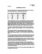
The tally charts above show us the mode, or the most recurrent class interval. For height the most common class interval is 1.5 ? h < 1.6. For weight the mode is 40 ? w < 50. The measurements are in meters and kilograms respectively. We can also now calculate the mean and find the median amongst our tally charts.
The median is the class interval in which the average of the 20th and 21st number is present.
Median of Height: 1.6 ? h < 1.7
Median of Weight: 50 ? w < 60
Mean of Heights:
(1.64+1.51+1.68+1.53+1.6+1.57+1.56+1.58+1.52+1.61+1.32+1.9+1.73+1.541.6+1.61+1.72+1.5+1.73+1.62+1.5+1.5+1.7+1.52+1.58+1.6+1.65+1.62+1.7+1.75+1.77+1.89+1.55+1.67+1.79+1.91+1.75+1.83+1.52+1.65) / 40
= 1.64m is the mean height for the pupils of Mayfield High School.
= 1.6 ? h < 1.7 is the class interval in which the mean for height lies in.
Mean of Weights:
(50+45+40+48+60+45+57+43+43+52+35+60+59+52+74+48+50+45+62+40+70+39+47+52+50+48+45+45+60+57+80+64+48+48+45+82+68+60+38+52) / 40
=52.65kg / 53kg is the mean weight for the pupils of Mayfield high School.
=50 ? w < 60 is the class interval in which the mean for weight lies in.
The mean and median correspond by appearing in the same category for weight and height but the mode is lower in both cases. This could be because there are more exceptions from the most frequent height and weight class interval.
Now it will be easy to construct my histogram from the data sorted out into class intervals in the previous tally charts for height and weight. I need to construct a histogram because the data for height and weight is continuous.
Now I will compare the different heights and weights between the girls and boys of Mayfield High School. This will give us a better idea of how different boys or girls are from the mixed trend of the entire school.
Firstly we will find out the mean median and mode for boys and girls by constructing separate Stem and Leaf diagrams and Tally charts.
Stem and Leaf Diagram for Heights of Boys and Girls
Boys
Stem
Girls
2
.30
.40
0, 0, 1, 3, 4
.50
0, 2, 2, 2, 5, 6, 7, 8, 8
0, 0, 2, 4, 8
.60
0, 0, 2, 4, 8
0, 0, 3, 5, 5, 7,
.70
2, 3, 9
9
.80
3
0, 1
.90
From the stem and leaf diagram above we can see that the boys have a more widespread distribution whereas the variance for girls is concentrated upon 1.5m to 1.7m. The mode for the boys is also higher than that of the girls.
Stem and Leaf Diagram for Weights of Boys and Girls
Boys
Stem
Girls
5, 9
30
8
0, 0, 5, 7, 8
40
3, 3, 5, 5, 5, 5, 5, 8, 8, 8, 8
0, 2, 7, 9
50
0, 0, 2, 2, 2, 7
0, 0, 0, 4, 8
60
0, 2
0, 4
70
0, 2
80
90
Again the weights of boys have a greater distribution than that of girls. The weights of the girls in my sample stay below 70kg possibly due to health consciousness and social awareness at this age whereas the boys are probably more carefree and easygoing. The girls have a mode but boys do not because modes do not have a value when more than one set of data has the same frequency as in this case.
Now I will construct the tally charts of boys and girls in the same manner.
Tally Chart for the Heights of Boys and Girls
Boys
Girls
Frequency
Tally
Class Interval
Tally
Frequency
.3 ? h < 1.4
.4 ? h < 1.5
5
.5 ? h < 1.6
9
5
.6 ? h < 1.7
7
6
.7 ? h < 1.8
3
.8 ? h < 1.9
2
.9 ? h < 2.0
Tally Chart for the Weights of Boys and Girls
Boys
Girls
Frequency
Tally
Class Interval
Tally
Frequency
2
30 ? w < 40
5
40 ? w < 50
1
4
50 ? w < 60
6
5
60 ? w < 70
2
2
70 ? w < 80
2
80 ? w < 90
To show the difference between the heights and weights of the boys and girls from the mixed heights and weights I will find out their individual means, medians and modes and tabulate the results.
Mean of Boys Heights:
(1.64+1.51+1.68+1.53+1.6+1.32+1.9+1.73+1.54+1.6+1.62+1.5+1.5+1.7+1.7+1.75+1.77+1.89+1.91+1.75) / 20
= 1.66m is the mean height for the Boys of Mayfield High School.
Mean of Girls Heights:
(1.64+1.51+1.68+1.53+1.6+1.32+1.9+1.73+1.54+1.6+1.62+1.5+1.5+1.7+1.7+1.75+1.77+1.89+1.91+1.75) / 20
= 1.62m is the mean height for the Girls of Mayfield High School.
Mean of Boys Weights:
(50+45+40+48+60+35+60+59+52+74+70+40+39+47+60+57+80+64+82+68) / 20
= 56.5kg / 57kg is the mean weight for the Boys of Mayfield High School
Mean of Girls Weights:
(45+57+43+43+52+48+50+45+62+52+50+48+45+45+48+48+45+60+38+52) / 20
= 48.8kg / 49kg is the mean weight for the Girls of Mayfield High School
Median of Boys Heights: 1.66m
Median of Girls Heights: 1.605m / 1.61m
Median of Boys Weights: 58kg
Median of Girls Weights: 48kg
Mode of Boys Heights: N / A
Mode of Girls Heights: 1.52
Mode of Boys Weights:
Mode of Girls Weights:
Table of results for Height (m)
Mean
Median
Mode
Boys
.66
.66
N / A
Girls
.62
.61
.52
Mixed Gender
1.64
.62
N / A
From the table above we can see that the Boys of Mayfield High School have a higher mean and median but we cannot see if this is the due to only a few extreme cases as there is no mode. The girls have a mean and median quite far from their mode so we can assume that there are a few girls who are much taller than other girls. The means and medians of boys and girls individually are quite close to the mean and median of them mixed.
Table of results for Weight (kg)
Mean
Median
Mode
Boys
57
58
60
Girls
49
48
45
Mixed Gender
53
50
45
From this table we can see that the mixed mean, median and mode are quite spread out. The mean, median and mode are clearly greater than that of the girls. However the difference between the mean, median and mode is small in the case of the girls and boys.
I will now draw a cumulative frequency graph to compare the heights and weights between boys and girls.
We can also compare the heights and weights of pupils through a frequency polygon graph. On this graph I will plot the heights and subsequently the weights of the boys, the girls and the mixed genders. This will allow us to see the various similarities and differences between girls, boys and all the pupils together.
I will now investigate the correlation between the heights and weights of the pupils of Mayfield High school. An effective way of showing the correlation between heights and weights is to construct a scatter diagram.
The scatter diagrams show that as the height of a person increases their weight increases as well (and vice-versa). The scatter diagram shows a strong positive correlation. However there are a few exceptions. These exceptions could be people who are big-boned and so weigh more than their weight, or people from a different country so genetic characteristics from that particular region could have influenced their height or weight in comparison with the rest of the pupils. To show a stronger correlation I will construct separate graphs for boys and girls.
The scatter diagrams again show that the distribution of the Boys is spread apart whereas the distribution of the Girls is concentrated. The two lines of best fit can be used to find a formula which can predict the weight of a pupil if given the height and vice versa.
In conclusion I have shown that the heights of people increased as their weights did (and vice-versa). I had said in my hypothesis that "boys will be spread apart more in terms of height and weight than girls." I have shown this at least within my own sample that Boys are taller and weigh more than girls and are more diverse in their heights and weights than girls. There may be some inaccuracies due to incorrect measuring or a few extreme cases that influence the entire sample. This extreme cases could be due to a variety of reasons some of which have stated along this coursework. To further extend this investigation I could have analyzed the data from different year groups as well as from different genders. I could also have found out the formula that would allow us to estimate the height of a boy / girl if given the weight and vice-versa.