Cumulative Frequency
In data handling the frequency tells you how often a particular result was obtained. Cumulative frequency indicates how often a result was obtained which was less than ( ) or less than or equal to ( ) a stated value in a collection of data.
Cumulative frequency can only be used when information has a clear order, such as measurements of height, age, weight, or quantities such as number of goals scored etc.
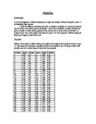
Below I have drawn tables showing the frequency and cumulative frequency of weights and heights for boys and heights and weights for girls.
The above table shows the cumulative frequency of the heights of the 30 boys. The data will be plotted onto a cumulative frequency graph.
The above table shows the cumulative frequency of the weights of the 30 boys. This data will also be plotted onto a cumulative frequency graph.
The above table shows the cumulative frequency for the heights of the 30 girls. This data will be plotted onto a cumulative frequency graph.
The above table shows the cumulative frequency for the weights of the 30 girls. This data will also be plotted onto a cumulative frequency graph.
As you can see from my above tables I have grouped the original data and arranged them into what are called class intervals I have grouped the data in classes of 10 to indicate more thoroughly how the heights and weights are spread as mentioned previously. My graphs will be shown on the next page.
Calculating the mean
To calculate the mean I would normally add up all the values for height or weight and then divide by the total number of values (in this case the 30 boys or 30 girls). I cannot do that with this information because I am using a value that is between say 30 or 40 and exactly what the value is. With grouped data like this I must use the middle value of each class interval and multiply by the frequency for that class interval. Then I will find the sum of the mid-values multiplied by the frequencies and divide that number by the total frequency. Note: to find the mid-value you must add the upper and lower value of the interval and divide by 2.
Mean= Total (mid-value x frequency)
Total Frequency
The data below shows the heights of the 30 boys.
Total=35 Total=60.15
Mean= Total (mid-value x frequency)
Total Frequency
=60.15 =1.72
35
Modal group= class with the highest frequency
Modal group = 1.65
The mid-value of the modal class gives an approximate value for the mode.
Median Class= class which contains the middle value= 1.65
The mid-value of the median class gives an approximate value for the median.
Range= maximum value (upper boundary of highest class) – minimum value (lower boundary of lowest class)
Range = 2.10-1.30= 0.8
The data below shows the weight of the 30 boys
Total= 34 Total= 1,940
Mean= Total (mid-value x frequency)
Total Frequency
= 1940= 57.06
34
Modal Group = 50-60 approximate mode = 55
Median group= 50-60 approximate median = 55
Range= 90-30 = 60
The data below shows the heights of the 30 girls
Total= 34 Total= 56.5
Mean= Total (mid-value x frequency)
Total Frequency
Median group= 1.60-1.70 approximate median= 1.65
Modal group= 1.60-1.70 approximate mode= 1.65
Range= 1.90-1.50 = 0.4
The data below shows the weights of the 30 girls.
Total = 33 Total = 1,675
Mean= Total (mid-value x frequency)
Total Frequency
= 1675 = 50.76
33
Median group = 40-50 approximate median = 45
Modal group = 50-60 approximate mode = 55
Range = 70- 30 = 40
As you can see from the cumulative frequency graphs I have labelled 3 parts in particular. The median, lower quartile, upper quartile each of which is explained below.
Median
To find the median (middle number) of a set of data you would usually arrange the values in ascending numerical order and find the middle value. If n is the total number of values then the median is ½(n+1) value.
This suggest that to find median from a cumulative frequency curve you find ½(n+1) on the vertical axis (where n is the total frequency), draw a horizontal line to the curve and read off the corresponding value from the horizontal axis.
Upper, Lower quartile and Interquartile range
Knowing the range of a frequency distribution only tells me the extreme values. To see how the data are distributed around the median, the range is divided into four quarters.
The value one quarter of the way from the lower end of the range is called the lower (or first quartile). The middle value or the second quartile is the median itself. The value three quarters of the way from the lower end of the range is called the upper (or third quartile).
If the total frequency, n, is large then the first quartile has cumulative frequency ¼n and the third quartile is at ¾n. If n I small then the first quartile is at ¼(n+1) and the third quartile is at ¾(n+1).
The difference between the lower and upper quartiles is called the interquartile range. In any frequency distribution half of the data lies within the interquartile range. This is a very useful way to measure the spread of a set of data, since it only includes the half of the data, which is closest to the median, and avoids distortions caused by unusually large or small values. There are a number of more accurate ways in which one can measure the spread of a set of data. One of the more precise ways is shown in the next section.
Deviation from the mean
The distance of a value from the mean is called its deviation from the mean. Due to my data being grouped I will now use the original data to get an exact deviation from the mean rather than an estimate. First to find the mean I will add up all the heights for the 30 boys and divide by 30.
Looking at the above table you can see that there are three columns one of which you may not understand as of yet. The third column is called the deviation. It is found by subtracting the mean () from each of the values in the height column (x).
Mean Deviation
If you try and find the mean of the deviations in the usual way you will find that your answer equals zero.
Finding the mean of the deviations in this way takes into account, which side of the mean the values are (i.e. whether the deviation is positive or negative). But this is not necessary.
To make the values more useful just consider the size of each deviation and ignore the direction. This positive value is called the modulus (sometimes shortened to mod) and is written like this:
x-
The mean size of the deviation can now be calculated.
Mean Deviation = x-
N
The sign means sum of (add up) all the values. N is the number of values, which have been added.
Therefore the mean deviation of the heights of the 30 boys is: 0.38+0.25+-0.15+0.15+0.15+0.14+0.2+0.41+0.08+0.04+0.31+0.13+0.14+0.21+0.31+0.56+0.23+0.18+0.23+0.33+0.37+0.2+0.24+0.05+0.25+0.44+0.3+0.33+0.39+0.34 = 7.19
7.19 =0.24
30
So the average distance of the values from the mean is 0.24
Variance
An alternative way to get positive values for the deviation from the mean is to square the deviation. The squares of the deviations can now be added and their mean value calculated. This mean of the squares of the deviations is called the variance.
Variance = (x-) ² Where n is the total number of values.
N
Variance = 2.30 = 0.076666666
30
Since the original problem was to measure the spread of the heights of the 30 boys, an answer of 0.076666666 does not seem to make much sense. This is because the deviations were squared. This can be corrected by taking the square root of the variance.
Standard Deviation
The Square root of the variance is called the standard deviation. The standard deviation is given by
= (x-) ²
n
For the heights of the 30 boys the standard deviation is 0.076666666
= 0.28 (to 2.d.p)
Now I can add my standard deviation to my mean and subtract my standard deviation from my mean. This tells me the measure of spread is between:
1.19m and 1.75m.
I can now do three more tables similar to the one above to find out the standard deviation for the weight of the 30 boys and the height and the weight of the 30 girls.
The table below shows the data for the weight of the 30 boys.
Total = 4610.8
4610.8 = 153.69
30
Standard deviation = 153.69
= 12.4
Now I can add my standard deviation to my mean and subtract my standard deviation from my mean. This tells me the measure of spread is between:
46.4kg and 71.2kg
The table below shows the data for the height of girls
Total =0.1493
0.1493/30 = 0.004976
Standard Deviation = 0.004976
= 0.07
Now I can add my standard deviation to my mean and subtract my standard deviation from my mean. This tells me the measure of spread is between:
1.6m and 1.74m
The table below shows the weight data for the 30 girls.
Total= 993.5
993.5 = 33.1
30
Standard Deviation = 5.76
Now I can add my standard deviation to my mean and subtract my standard deviation from my mean. This tells me the measure of spread is between:
44.3kg and 55.86kg.
Stratified Sampling
Stratified sampling involves dividing the population into groups or strata. From each stratum I would choose a random or systematic sample so that the sample size is proportional to the size of the group in the population as a whole. For example, in a class where there are twice as many girls as boys, the sample would have to include twice as many girls as boys. Below I shown how I would have used stratified sampling if I had done so from the beginning of the investigation.
The total population is 1183.
If I decide I would like to sample 100 people from the school then I would need to find out how many girls and boys I would be taking from each year. Below I have shown how I would do this. Rather than just taking 30 boys and 30 girls from year 11.
The number of boys in year 10 is 106.
As a proportion of the total of 1183 this is 106/1183 = 0.09 (to 2d.p).
My total sample is to be 100 so I would sample:
0.09 x 100 = 9 boys from year ten.
The number of girls in year 10 is 94.
As a proportion of the total of 1183 this is 94/1183 = 0.08 (to 2d.p).
My total sample is to be 100 so I would sample:
0.08 x 100 = 8 girls from year ten.
The number of boys in year 11 is 84.
As a proportion of the total of 1183 this is 84/1183 = 0.07 (to 2d.p).
My total sample is to be 100 so I would sample:
0.07 x 100 = 7 boys from year eleven.
The number of girls in year 11is 86.
As a proportion of the total of 1183 this is 86/1183 = 0.07 (to 2d.p).
My total sample is to be 100 so I would sample:
0.07 x 100 = 7 girls from year eleven.
Conclusion
I think that the statistical investigation turned out very successful. I was able to compare my results using scatter diagrams and I managed to find a standard deviation from the mean. I think that the methods I used have given me some strong results to comment on. After having done the scatter diagrams I immediately realised that the taller the children were the more they weighed, in most cases. The graphs showed a positive correlation. I think that most accurate statistical method I used was standard deviation. It showed quite clearly the measure of spread for the different data that I used. The next time I carry out an investigation such as this one, I think that I may use stratified sampling, as it is a very strong way of reading statistics. I would facilitate me to write a stronger conclusion than I have.