Range = largest value – smallest value
The table above shows that all averages for boys are greater than girls; therefore it proves my hypothesis that boys of the whole school are heavier than girls.
Range for girls is greater than for boys, the reason for it could be an anomalous value that one girl weigh 140 kg.
Now I am going to find variance and standard deviation to see how spread the data is between the weights of boys and girls. Standard deviation (s) is the square root of variance (s2).
68% of the values lie within 1 standard deviation of the mean
95% lie within 2 standard deviations of the mean
99.75% lie within 3 standard deviations of the mean
The 2 standard deviation test is a way of defining outlier. If the value is ± 2 standard deviations above the mean, that value is called an outlier.
Boys:
Mean (ā) = ∑fa/∑f = 3124/58 = 53.86 kg
n = ∑f
Standard deviation (s) = √(∑fa2 – nā2)
√(n - 1)
= √(176750 – 58 x 53.862)
√(58 - 1)
s = 12.2
Variance (s2) = 148.84
Lower end = 53.86 – 2 x 12.2 = 29.46
Upper end = 53.86 + 2 x 12.2 = 78.26
26 < 29.46 therefore 26 is an outlier.
92 > 78.26 therefore 92 is an outlier.
Girls:
Mean (ā) = ∑fa/∑f = 2969/59 = 50.32 kg
Standard deviation (s) = √(∑fa2 – nā2)
√(n - 1)
= √(160139 – 59 x 50.322)
√(59 - 1)
s = 13.6
Variance (s2) = 184.96
Lower end = 50.32 – 2 x 13.6 = 23.12
Upper end = 50.32 + 2 x 13.6 = 77.52
There is no outlier at lower extreme, but 140 is an outlier at upper extreme because 140 > 77.52.
Variance for girls is greater than for boys, it mean the weight of girls is more varied. The reason for it can be due to an outlier at upper extreme.
Year 7:
n = 28, but there is one value missing in the data for a male weight therefore n = 27.
Male
n = 14
32, 38, 42, 43, 44, 48, 50, 50, 50, 53, 56, 57, 57, 59
Female
n = 13
38, 38, 40, 42, 45, 45, 47, 47, 49, 50, 50, 51, 140
Key 30|2 = 32
The table above shows that all averages for boys are greater than girls; therefore it proves my hypothesis that boys of the year 7 are heavier than girls.
Range for girls is greater than for boys, the reason for it could be an anomalous value that one girl weighs 140 kg.
Boys:
Mean (ā) = ∑fa/∑f = 679/14 = 48.50 kg
Standard deviation (s) = √(∑fa2 – nā2)
√(n - 1)
= √(33745 – 14 x 48.502)
√(14 - 1)
s = 7.91
Variance (s2) = 62.57
Lower end = 48.50 – 2 x 7.91 = 32.68
Upper end = 48.50 + 2 x 7.91 = 64.32
32 < 32.68 therefore 32 is an outlier. There is no outlier at the upper extreme for year 7 boys.
Girls:
Mean (ā) = ∑fa/∑f = 682/13 = 52.46 kg
Standard deviation (s) = √(∑fa2 – nā2)
√(n - 1)
= √(44322 – 13 x 52.462)
√(13 - 1)
s = 26.68
Variance (s2) = 711.8
Lower end = 52.46 – 2 x 26.68 = -0.9
Upper end = 52.46 + 2 x 26.68 = 106.06
There is no outlier at lower extreme, but 140 is an outlier at upper extreme because 140 > 106.06. This outlier affects standard deviation, variance and mean.
Year 11:
n = 17
Key 50|8 = 58
Boys
n = 8
50, 58, 60, 63, 66, 68, 72, 92
Girls
n = 9
44, 48, 51, 51, 52, 52, 54, 55, 60
The table above shows that all averages for boys are greater than girls; therefore it proves my hypothesis that boys of the year 7 are heavier than girls.
Range for boys is greater than for girls, so it strengthens more my hypothesis.
Boys:
Mean (ā) = ∑fa/∑f = 529/8 = 66.13 kg
Standard deviation (s) = √(∑fa2 – nā2)
√(n - 1)
= √(36061 – 8 x 66.132)
√(8 - 1)
s = 12.43
Variance (s2) = 154.41
Lower end = 66.13 – 2 x 12.43 = 41.27
Upper end = 66.13 + 2 x 12.43 = 90.99
There is no outlier at lower extreme for year 11 boys, but 92 is an outlier at upper extreme.
Girls:
Mean (ā) = ∑fa/∑f = 467/9 = 51.89 kg
Standard deviation (s) = √(∑fa2 – nā2)
√(n - 1)
= √(24391 – 9 x 51.892)
√(9 - 1)
s = 4.44
Variance (s2) = 19.73
Lower end = 51.89 – 2 x 4.44 = 43.01
Upper end = 51.89 + 2 x 4.44 = 60.77
There is no outlier for year 11 girls.
The calculation above showed that the weight of the girls is less than boys. Therefore it strengthens my hypothesis.
Weight comparison of different aged groups:
Year 7
n = 27
32, 38, 38, 38, 40, 42, 42, 43, 44, 45, 45, 47, 47, 48, 49, 50, 50, 50, 50, 50, 51, 53, 56, 57, 57, 59, 140
Year 11
n = 17
44, 48, 50, 51, 51, 52, 52, 54, 55, 58, 60, 60, 63, 66, 68, 72, 92
The table above shows that all averages for year 11 are greater than for year 7; it shows that as pupils grow their weight increases.
Range for year 11 is less than for year 7; it could be due to anomalous weight of a year 7 female.
Year 7:
Mean (ā) = ∑fa/∑f = 1361/27 = 50.41 kg
Standard deviation (s) = √(∑fa2 – nā2)
√(n - 1)
= √(78067 – 27 x 50.412)
√(27 - 1)
s = 19.07
Variance (s2) = 363.67
Lower end = 50.41 – 2 x 19.07 = 12.27
Upper end = 50.41 + 2 x 19.07 = 88.55
140 > 88.55 therefore 140 is an outlier. There is no outlier at lower end.
Year 11:
Mean (ā) = ∑fa/∑f = 996/17 = 58.59 kg
Standard deviation (s) = √(∑fa2 – nā2)
√(n - 1)
= √(60452 – 17 x 58.592)
√(17 - 1)
s = 11.44
Variance (s2) = 130.9
Lower end = 58.59 – 2 x 11.44 = 35.71
Upper end = 58.59 + 2 x 11.44 = 81.47
There is no outlier at lower extreme, but 92 is an outlier at upper extreme because 92 > 81.47.
Mean weight for year 11 is greater than for year 7, it means as pupils grow their weight also increases. Standard deviation for year 7 is larger than for year 11, the reason for this result is outlier at upper extreme. The outlier 140 for year 7 is bigger than the outlier 92 for year 11, therefore it affects the standard deviation the most and thus variance is also affected.
Weight comparison between females of different ages:
Year 7 females
n = 13
38, 38, 40, 42, 45, 45, 47, 47, 49, 50, 50, 51, 140
Year 11 females
n = 9
44, 48, 51, 51, 52, 52, 54, 55, 60
The table above shows that modal class and median for year 7 females are less than for year 11. Other values range, mean, standard deviation and variance are larger for year 7; it is due to a huge outlier at the upper extreme of year 7 females. Year 11females contain no outlier therefore the data is unaffected.
Weight comparison between males of different year groups:
Year 7 male
n = 14
32, 38, 42, 43, 44, 48, 50, 50, 50, 53, 56, 57, 57, 59
Year 11 male
n = 8
50, 58, 60, 63, 66, 68, 72, 92
The table above shows that all of the averages for year 7 males are less than for year 11 males, despite of containing an outlier for each year group. Data for year 7 males has an outlier at the lower end and for year 11 males there is an outlier at the upper end, therefore the results are not influenced.
Hypothesis 3:
As pupils’ age increases, the pupils’ height increases as well.
I separately drew box and whisker plot for each year group to compare their heights on the same axis. Box and whisker plot is drawn to show how spreads out the values are and to find any outliers which affect the skewness. If any value is out of the range of 25% or 75% of the data, it is called an outlier.
- Firstly I put heights of students for each year group in numerical order.
- Then I worked out the median for each year group. Median is the middle value of the data.
- In normal symmetrical distribution, mean mode and median are same. In box and whisker plot, median is in the middle and lower quartile and upper quartile are on the each end of the box with the same distance from the median. The curve and diagram below show normal distribution.
- If median is in the middle of the curve and mode moves to left and mean moves towards right then distribution is positively skewed. In box and whisker plot, if median is closer to lower quartile than upper quartile then distribution is positively skewed.
- If median is closer to upper quartile than lower quartile then distribution is negatively skewed. In a curve, if mode moves to right of the median and mean towards right then distribution is negatively skewed.
-
For year 7, n = 28. The n value is even, the half of 28 is 14. To find out median, I will halve the sum of 14th and 15th height. The data is given below.
1.45, 1.46, 1.47, 1.48, 1.49, 1.51, 1.51, 1.52, 1.53, 1.54, 1.55, 1.55, 1.55, 1.57, 1.57, 1.59, 1.59, 1.6, 1.61, 1.62, 1.63, 1.63, 1.64, 1.64, 1.66, 1.69, 1.70, 1.73
14th value is 1.57 and 15th value is 1.57
Therefore
Median height (Q2) = (1.57+1.57)/2 = 1.57m
-
Lower quartile Q1 is the average of the middle two values of the 1st 1/2 of the data, because first half contains 14 values.
1.45, 1.46, 1.47, 1.48, 1.49, 1.51, 1.51, 1.52, 1.53, 1.54, 1.55, 1.55, 1.55, 1.57
In this case lower quartile is the average of 1.51 and 1.52.
Q1 = (1.51+1.52)/2 = 1.515
-
Upper quartile Q3 is the average of the middle two values of the 2nd half of the data, because the second half also consists of 14 values.
1.57, 1.59, 1.59, 1.6, 1.61, 1.62, 1.63, 1.63, 1.64, 1.64, 1.66, 1.69, 1.70, 1.73
Upper quartile is the average of 1.63 and 1.63.
Q3 = (1.63+1.63)/2 = 1.63
-
Inter quartile range = Q3 – Q1 = 1.63 – 1.515 = 0.115
-
Outliers are any points below Q1 or above Q3. Outlier = Q1 – 1.5×IQR and outlier = Q3 + 1.5×IQR
- For year 7
Outlier = 1.515 – 1.5 x 0.115 = 1.3425
Outlier = 1.63 + 1.5 x 0.115 = 1.8025
For year 7 there is no outlier because no value is less than 1.3425 or greater than 1.8025.
The diagram above shows different types of distribution.
The reason for having an outlier could be because of noting figure wrongly. Mean is mostly affected due to an outlier. Distribution shows that how spread the data is around median. Each box and whisker plot shows that how height varies in different year groups. As I look at the means across all year groups, it shows that pupils’ mean height increases except year8. The reason for this odd mean result could be because of bimodal data. If I compare the mean heights of year7 and year11, year11 students are taller than year7, therefore my hypothesis is proved.
Overall conclusion:
I can conclude that whatever I had decided to investigate considering year groups, weight, height and gender. I think that I have been successful in achieving the results. The only fact which affected my results the most that the weight of one year7 male.
- Sampling
- I had decided to choose 10% of the sample using stratified, random and systematic sampling.
- 10% of the sample of 1183 pupils was equal to 118 pupils.
-
I easily found the sample of 118 students, for it I chose every 8th pupil using systematic sampling.
- Hypotheses
I decided to set up three hypotheses to find different combinations between weights and heights, differences of weights and heights considering genders and different aged groups.
2a. Hypothesis 1
- For hypothesis1 I said that the pupils’ weight would increase because their height would increase.
- To prove my hypothesis I drew a scatter diagram of height(m) and weight(kg) for the whole school. It showed a positive correlation which strengthened my hypothesis. Then I found Pearson’s correlation coefficient using Microsoft excel to see how strong my hypothesis’s correlation was.
- To analyse data in more depth, I found the relationship of height(m) and weight(kg) between different aged groups. I considered year8 and year11.
- I drew scatter diagrams separately for year8 and year11 considering height(m) and weight(kg) and I also found Pearson’s correlation coefficient for them.
- Both diagrams showed that pupil’s weight would increase with their increasing heights.
- Pearson’s correlation coefficient for year11 was higher than for year8.
- This hypothesis also proved that as pupils would get older, their weight would increase with their increasing height.
2b. Hypothesis 2
- For hypothesis2 I said that boys would weight more than girls. There was one value of the weight for year7 male was missing; it affected my results the most.
- To start investigation, I separated the data of weights for males and females and then put it in numerical order.
- To make calculation easier I drew a tally table to see how much data would lie in each class. It helped in estimating the class in which mean, median and modal class would lie.
- I drew back to back stem and leaf diagram to compare the weights of boys and girls for the whole data.
- Using stem and leaf diagram I found modal class, mode, mean and median for boys and girls. It showed that all results for girls were smaller than for boys. It made my hypothesis stronger that boys are heavier than girls.
- Then I calculated the range which was greater for girls than for boys, it was because of the outliers who mostly affect mean, range, standard deviation and variance. Median and mode are not affected by outliers.
- There were two outliers for boys’ data and one outlier for girls which was a large outlier.
- Standard deviation for girls was greater for girls than for boys; the reason for it was an outlier 140 which affected the standard deviation a lot. It showed that the data for girls was more spread.
- Variance showed how variation of the data. The variance value for girls was greater than for boys; it was because of the large standard deviation for the girls.
- The only thing which weakened my hypothesis was outlier.
- I repeated the same calculations to find different relationships between the weights of year7 and year11 considering aged factors including different genders, gender factors and aged factors involving same gender.
- I firstly investigated the relationship between weights of year7 males and females. It showed that modal class and median for boys were larger than for girls; it made my hypothesis stronger that boys are heavier than girls, but the range, mean, standard deviation and variance for girls was greater than for boys due to presence of a big outlier 140(kg).
- I repeated the same investigation for the weights of year11 males and females. It showed that modal class, mean, range, median, standard deviation and variance for girls were smaller than for boys, because there was no outlier for year11 girls but there was only one outlier 92 for year11 boys; therefore the data was less distressed. It strengthened my hypothesis that boys weigh more than girls.
- I found the relationship of weights between different aged groups. It demonstrated that the data for year 7 was bimodal. The mode, median and mean for year7 were lower than for year 11. It proved that as pupils would grow their weights would increase with their increasing heights (hypothesis1). The range, standard deviation, and variance for year11 were less than for year 7 because of the outlier140 for year7.
- Then I observed the relationship of the females of different aged. Modal class and median for year7 females were less than for year11; it helped in making my hypothesis strong. The range, mean, standard deviation and variance for year7 were greater than for year11 because one year7 female weighed 140kg. That was the only reason which affected my hypothesis2 overall.
- Then I learnt the correlation of the different aged males. All of the results such as range, mean, modal class, standard deviation and variance for year11 males were greater than for year7 despite of containing an outlier for males of each year group.
- The overall conclusion that I can see is that the outlier for year7 females weakened my hypothesis. Otherwise the outliers for males had no effect.
2c. The third hypothesis I set up was that the pupils’ height would increase with their increasing age.
- To see combination, I drew box and whisker plots for the heights(m) of each year group separately to see the distribution of the data. It showed that the data for year8 was highly distributed.
- Then I drew a table representing number in sample, mean, mode, median, lower quartile, upper quartile, inter quartile range, distribution and outliers.
- Median height(m) increased as year group increased except for year10, it gave strength to my hypothesis.
- Modal heights for year7 and year10 were the same. Year8 was bimodal and modes for year10 and year11 were larger than others.
- Mean height increased as year group increased except for year8; it could be due to 2 modal heights for year8.
- The distribution for year7 was symmetrical, for year8, 9 & 10 was positive and for year11 was negative. It affected the inter quartile range.
- The inter quartile range was affected by outliers. There was no outlier for year7, 8 & 10. For year 9 there was one outlier 1.06m and for year 11 there were three outliers 1.52m, 1.79m & 1.82m; these outliers affected the distribution of the data.
The overall result shows that I have not been completely successful in proving my hypotheses. The outliers and some anomalous values affected the distribution of the data. There was one weight value missing which also affected the results to prove my hypotheses. For different samples the results would be different. So the same results can’t be assumed for different sample.