Female:
The histogram displaying the number of minor mistakes made by my female sample shows an uneven pattern, were all the bars are of various heights. The histogram again shows that the majority of female drivers did complete their driving test with less than half of the possible amount of minor mistakes awarded, but the female columns described in this histogram do not maintain their majority for as long as the males did. The female majority is not as big in comparison with the male majority. So the first three bars are large and do contain the majority for the female histogram. Again after the three first columns there is a sharp drop again suggesting that the small minority of females in the last three columns obtained a high number of minor mistakes. My frequency polygon also backs this up.
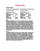
Driving Tests
Statistical Comparison:
Mean:
The mean displayed for both genders in the above statistics are very close. But the male mean is still smaller at 13.125 to the females 13.4375. The smaller mean held by the male sample signifies that they as a sample produced a smaller average amount of minor mistakes than the female sample.
Standard deviation:
The standard deviation helps one to know how a set of data clusters or distributes around its mean.
In the male case the standard deviation is 8.28685 this means that the majority of the results in the box plot and histogram fluctuate around the mean of 13.125 plus or minus 8.28685. In the women’s case the standard deviation is 7.36732 and therefore fluctuates around their mean of 13.4375 plus or minus 7.36732.
This means that the majority of the male results are found between (13.125 – 8.28685, 13.125 + 8.28685) 4.83815 and 21.41185.
In the female case the majority of the female results are found between (13.4375 – 7.36732, 13.4375 + 7.36732) 6.07018 and 20.80482.
We cannot solely rely on the standard deviation to determine a conclusion as the results are quite vague, but we can see that the male lower boundary is lower than the females and therefore the majority of their results could be lower than the females. On the females argument we can see that their upper boundary is lower than that of the male upper boundary but to a lesser extent than the difference between the lower boundaries and therefore the standard deviation would suggest vaguely that the males made less mistakes.
Range:
In the case of ranges, the females have obtained a higher range by 2 mistakes. This difference means that a female within the female sample obtained the largest amount of minor mistakes out of the two samples. We do not know how many received 32 mistakes but we know that one female did, and this result would back up the mean, suggesting that females are not as good drivers as males.
Lower quartile:
The lower quartile is a value for which 25% of the observations are smaller and 75% are larger. In the statistics above we can see that the female sample produced a slightly larger lower quartile of 8.25 against the males 8.00. Again the odds are stacked in the males favour. The females having the higher lower quartile means that 25% of their observations are lower then 8.25, were the male observations have 25% under 8.00 mistakes made, which is slightly smaller than the females.
Median:
The median is the middle value in an ordered array of data, were half the observations will be smaller than the median and half will be larger. On comparing the two sets of statistics we can see that the male median is slightly smaller at 12.5 than the female median at 13.0769. Thus due to the males smaller median we have another factor that backs up that the male sample made less mistakes than the females, because half are below and above 12.5 whereas the females have half below and above 13.0769.
Upper quartile:
The upper quartile is a value for which 75% of the observations are smaller and 25% are larger. On this occasion the males have a larger upper quartile of 18.333, and the females have a lower upper quartile of 17.5. So because the females have a smaller upper quartile it would mean that 75% of their observations are below a number that is smaller than that of the male sample. Suggesting that females are making less mistakes than the males, but this factor is not very precise as we do not know how the observations a re distributed within the 75%.
Semi inter-quartile range
The semi inter-quartile range measures the distance from the middle of the distribution to the boundaries that define the middle 50%. We can see that the females have a smaller semi inter-quartile range of 4.58333 than the males’ semi inter-quartile range of 6.04167. This means that the males having a lower semi inter-quartile range have the majority of their distributions 6.04167 below the 50% boundary and therefore have more observations with less mistakes.
Driving Tests
Conclusion:
Box and whisker analysis:
What I can see from the statistics described in my two box plots are that men make less mistakes than women do, this is because among other factors, the female median and mean are larger than that of the male one. But the median can be easily swayed, and in the female case the median could be larger due to the females upper class value. Also, since both my charts are quite alike it is difficult to suggest an evidential judgement.
I also created four more box and whisker diagrams. I compared the male and female samples with their populations. We can see from the diagrams that in both cases the medians are fairly close to each other (male, medians 13.5, 12.5) (female, medians 17, 14) and therefore this proves that my samples are not biased.
Histogram analysis:
The histograms shown both depict similar results and follow a similar pattern, which makes a conclusion difficult to judge. It is difficult to get an exact or firm conclusion from these results because the two graphs are closely linked. But what I can see from the statistics described in my two histograms and the general look of the histograms are that men make less mistakes than women do and so are better drivers.
Statistical comparison:
The majority of the various statistical measures described are in favour of the males being the ones that made fewer mistakes. Although there are one or two statistics such as the upper quartile that would reveal that the females made fewer mistakes.
Result:
From the results acquired from hypothesis one, I believe at the moment that the males are the better drivers and do make less mistakes because the large majority of diagrams and statistics so far would suggest that way, but we do not know for sure. The females are favoured on a few occasions, but I have noticed that the values deciding who is favoured have been extremely close, and so this maybe due to rogue results or similar happenings or other factors which we have not investigated. Most of the information points towards the males as being the better drivers than the females and so to answer the hypothesis I would say that males are better drivers than the females. Still it is uncertain and I must continue my investigation to collect results from other factors that would help me to affirm an evidential conclusion.