Stratified sampling graph
The graph below is my stratified sampling graph which will help me get a proportionate number to chose from out of the data of both gender and year group. Therefore the data I end up with in the end will reflect the amount of people in each year group and each gender.
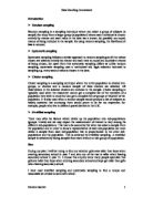
By looking at the graph above you are able to see that there is a positive correlation between year group and height since the older the girls were in the enquiry the taller they got.
As you can see in the scatter graph above you are able to see that there is a positive correlation between year group and height since the older the boys were in the enquiry the taller they got.
Furthermore by comparing the line of best fit for both graphs we can see that boys are taller than girls at the start middle and end of secondary, this is shown by the fact that the line of best fits of boys start year seven at an average height of 1.50 while the girls is only 1.45, this trend continues year by year and in year 11 the average boys height shown by the line of bit fit is 1.75 while the girls is 1.70. Consequently this mean that at the start, middle and end of secondary school boys are always taller which proves wrong the theory that girls are taller than boys at the beginning of secondary school while boy are taller at the end. However there are many other ways to test this theory and since I only used one I could be would, but I am choosing not to continue with the plan but to move on to something similar
Handling Data Coursework
For my data handling coursework I was be doing an enquiring on whether the BMI body mass index of boys is larger than that of girls and whether the taller you are the or heavy you are affects how high your BMI is. During this coursework I will be following the same steps as I did during the plan but I will be expanding the means of analysing the data that I will chose using the same two method of sampling as before. This will be done by doing a frequency table and doing a cumulative frequency graph as well as many other methods. Body mass index (BMI) is measure of body fat based on height and weight that applies to both adult men and women.
Method to calculate BMI is: BMI = Weight (kg) / Height (m) 2
Prediction
I predicted from my knowledge priory to this investigation that the BMI of boys would be higher than that of girls since boys are generally heavier giving them a higher BMI even if they are taller than girls. I also predict that as year group (age) increase so will BMI for both girls and boys since both gender generally get heavier as they grow older.
Stratified sampling graph
The graph below is my stratified sampling graph which will help me get a proportionate number to chose from out of the data of both gender and year group. Therefore the data I end up with in the end will reflect the amount of people in each year group and each gender.
We can see in the scatter graph above that there is a large negative collection between BMI and height meaning that as height increases BMI decreases which prove my prediction that as BMI will decrease as height increases. I believe this comes as a result of height being the denominating factor in the equation to calculate BMI therefore if you are increasing the height the BMI wall fall.
We can see in this scatter graph that there has been a similar outcome to that of the girls although the negative correlation isn’t as big, I believe this is because even though if you increase height the BMI should fall weight is still a factor and if the weight is already high the BMI wouldn’t fall as quickly as it should especially if everyone is heavy and of similar weight.
With this scatter graph involving weight rather than height we can see that there is a positive correlation indicating that as weight increases so does BMI which I have announce in my prediction this is because weight is the numerating faction in the equation to calculate BMI and therefore as it increases BMI also increases since the numerator is increasing while the denominator stays the same making the result of the equation, the BMI, bigger.
This same theory about increasing weight directly increases BMI applies to this scatter graph as well since we can see as the boys weights increased so did the BMI.
In the scatter group above we can see that for girls as the grow order (increasing year group) there BMI decrease as you can see a negative correlation between BMI and year group on the scatter graph above. I believe this to be a result of girls either getting taller or losing weight as they grow up as these are the two variable involved in calculating BMI.
However for the boys in the scatter graph above there seems to be a small positive correlation between year group and BMI meaning that the boys as they are getting older are getting heavier since they cannot get shorter to increasing their BMI.
Mean = ∑ fx / ∑ f
= 487.5 / 50
= 19.5
Using the equation above I have found out that the average of BMI for all the girls I studied is 19.5 telling me that most of the girls that I studied were in normal zone for weight status since their average BMI of 19.5 is between 18.5 – 24.9, meaning that mostly every I studied was not under or overweight.
Standard Deviation = √ [ ∑ fx2 / ∑f – ( ∑fx / ∑f ) 2 ]
= √ [9906.5/ 25 – ( 487.5 / 25) 2 ]
= 4
Since the standard deviation of the girls BMI is relatively small I can say that there is a small spread around the mean since mostly all the BMI’s of the girls I studied were clustered together resulting in them having a small spread around the mean.
Q1 = 17
Median / Q2 = 19
Q3 = 23
Inter quartile range / Q3-Q1 = 23-17 = 6
Highest point = 27.5
Lowest point = 12
Box Plot
As we can see in the box plot diagram above the spread for the BMI for girls is widely spread with a inter quartile range of 6 and median of 19 telling me that the girls BMI which I studied were widely spread with the highest being 27.5 and lowest 12 with a range of 15.5.
Histogram and Frequency polygon
For this particular histogram gram and frequency polygon showing the frequency density for girls BMI, tells me that the most of the girls in Mansfield school have a BMI between 15-22. This can be seen in the histogram, as the frequency density of the area between 1
5-22 is the largest telling us the girls BMI are concentrated in this area.
Mean = ∑ fx / ∑ f
= 517.5/ 25
= 20.7
Using the equation above I was able to find the mean of the boys BMI, which is 20.7 telling me that most of the boys in Mansfield school that I studied were not over or under weight since the average is in the norm of 18.5 – 24.9.
Standard Deviation = √ [ ∑ fx2 / ∑f – ( ∑fx / ∑f ) 2 ]
= √ [10956/ 25 – ( 517.5 / 25) 2 ]
= 3
The standard deviation question above tells me that the spread around the mean BMI for the boys is relatively small meaning that most of the boys BMI are concentrated around the mean.
Q1 = 18
Median / Q2 = 21
Q3 = 23
Inter quartile range / Q3-Q1 = 23-18 = 5
Highest point = 27.4
Lowest point = 15.1
Box plot
As we can see in the box plot diagram above the spread for the BMI for boys is evenly spread with a inter quartile range of 5 median of 21, this tells me that the boys have an evenly spread out BMI with the range of 12.3 apart for the highest to the lowest points.
Histogram and Frequency polygon
In the histogram above we are able to see that the frequency density for the boys is concentrated in the area between 16-22, telling me that most of the boys have BMI in this area since it will have a higher frequency when calculated.
Analysis
Through comparison of the box plots, histogram and standard deviations I was able to find out that the boys generally have BMI bigger than that of girls meaning they are either heavier or shorter but because of the information I gained through the scatter graphs telling me that boys are generally taller than girls it must mean the boys have a higher BMI because they are heavier.
We can immediately tell by comparing the two box plots for the boys and girls that most of the boys I studied have a higher BMI because their median BMI is 21 while the girls is only 19. However we can also see that the girls are more widely spread because of the fact that the range between their highest and lowest points is 15.7 compared to the boys 12.3.
Furthermore the graph above of a frequency polygon comparing the frequency density for both boys and girls, allows to see that the boys that I studied in my enquiry mostly have a BMI in the region of 16-22 since using the frequency density we are able to calculate the frequency which proves to be quite high in this region meaning the majority of boys I studied had a BMI in this region. However with the girls using the frequency density and class width I was able to find out that most of the girls I studied had a BMI in the region of 14-20 which can be seen in the frequency polygon above since the frequency is very high in this region meaning that most girls had BMI’s in that particular area. Consequently I believe that most of the boys had a BMI in the region higher than that of the girls since boys are generally heavier than girls and not tall enough to lower their BMI to that of girls.
Conclusion
In conclusion I have found out from carrying this enquiry that the boys were naturally taller than the girls, which can be seen in the scatter graphs I carried out in my plan. From this I used the knowledge I gained and changed the enquiry slightly to find out whether boys had a bigger BMI than girls since I knew that boys were taller but also heavy so I wanted to find out whether they will still have a bigger BMI than girls since they are taller and height reduces BMI while weight increases BMI.