A stem and leaf is made by putting the digits between 0- 10 in a vertical line. These represent the first digit in a number. For every value in the data set you place the number’s second digit in its corresponding first number of the diagram (e.g. the number 24 will be placed in the 2 bar and will put a 4 in it’s bar to represent its number). These numbers will be sorted so that they go in an increasing order.
I decided to use a mean because it shows me my entire set of data in one number. This though can be contorted by extreme values and so isn’t very reliable. The range is good because it shows how much difference there is between the highest and lowest value. This shows how much the data set varies but can again be distorted by extreme values and so isn’t too reliable. The standard deviation however tells me the average variation of the data values from the mean number. This can’t be contorted very easily because it takes into account every value and so is very reliable in telling me how much the values vary either way from the mean. The bar chart is useful because it compares in one graph each value. From it I can see the highest and lowest value quite easily and see how much the data varies.
Male adult illiteracy rate in 1990-
Mean= 3001/125= 24.008%
Range= 82-0.5= 81.5%
Standard Deviation= 123935-242 = 20.38%
125
Stem and Leaf Diagram- 0 000000111111122222234455566666778899
1 000000111233333333444578889
2 00222233347889
3 01111233444555667889
4 0011235779
5 00133344679
6 23478
7 5
8 2
Analysis-
The Mean of this data is quite high but is only just above the normal percentage for this column. This tells me that countries all around the world have a normal illiteracy rate in male adults in 1990. But that can only be said if the values do not vary too much but, looking at the standard deviation and the bar chart, I can tell they do.
Since the mean is low and looking at the stem and leaf diagram I can safely say that, although the values vary greatly, the bulk of the percentages are quite low.
The pie chart as you can see has very little use as there are too many values and no detailed analysis can be made of it. So, as a result, I will not do any further pie charts for the next parts of the data.
Male adult illiteracy rate in 1999-
Mean= 2371/125= 18.968%
Range= 77-0.5= 76.5%
Standard Deviation= 83212-192 = 17.45%
125
Bar Chart-
Stem and Leaf Diagram-
0 000000111111111222233334445555666667777778888899999999
1 01122234556677788899
2 0113346666677788999
3 1233344579
4 1111122456889
5 03477
6 7
7 7
Analysis-
The mean and standard deviation have both improved this year for the male adults. They have more lower illiteracy rate values than 9 years ago. This is especially evident in the stem and leaf diagram.
Female adult illiteracy rate in 1990-
Mean= 4679/125= 37.432%
Range= 95-0.5= 94.5%
Standard Deviation= 271781-37.52 = 27.71%
125
Bar Chart-
Stem and Leaf Diagram-
0 011111113334444555566678899
1 11122223445556677
2 00113555667778899
3 00012233499
4 12567999
5 0233466799
6 02234466678
7 123457799
8 000111246679
9 25
Analysis-
The Females have a much higher mean than males overall which tells me that they are more illiterate than men, but since their standard deviation is high I can’t make a proper judgement (their values are more spread out).
Looking at the bar chart you can see that there are generally a lot more high percentages than the males but the stem and leaf diagram is definitely more spread out than the males having a gradual, if varied, decrease in numbers from the top downwards. This pattern in the stem and leaf tells me that the females’ values are much more spread out than the males.
Female adult illiteracy rate in 1999-
Mean= 3779/125= 30.232%
Range= 92-0.5= 91.5%
Standard Deviation= 193285-30.22 = 25.18%
125
Bar Chart-
Stem and Leaf Diagram-
0 00011111122223333344455556677888999
1 0011111235566677799
2 00001112223445567
3 001123449
4 00111144567788
5 135555678
6 011355778889
7 012236679
8 27
9 2
Analysis-
The Females of each mentioned country have definitely decreased in their illiteracy rate overall since the past 9 nine years but comparing the means and standard deviations they are still higher than the males.
Again this is made much clearer in the bar chart and stem and leaf diagram. By comparing the two adult female bar charts you can see that they are very similar except that all the values have gone down, almost in ratio to each other. The stem and leaf diagram is also quite similar in the way the number of values decreases on the way down except that in 1999 it has much more values at the top than in 1990.
Calculations and graphs using cumulative frequency-
In this section I will convert all my data into a cumulative frequency table. This includes having a table with its first column including grouped values that corresponds to my data. So in this case it will be percentages and can be done in, perhaps, groups of 5’s. These groups would go all the way to my data’s maximum value, which will be 100% in this case. In the next columns I will place my types of data in a certain fashion. This fashion includes counting how many times a value from a certain data type occurs within the corresponding percentage group (e.g. the number of times a value occurs between 0-5% group in the male illiteracy rate in 1990 is 24). I will do this for every percentage group in every data type. This will give a frequency table. To get a cumulative frequency table I merely have to make a running total of the frequency. This should be done separately in each data type and if done properly you should get increasing values and the total of the amount of data at the end of the table. This is a cumulative frequency table.
With this data I can create a cumulative frequency graph and from this graph I can create a box plot, which shows me the median, the upper and lower quartile, the interquartile range and the skewness.
To create a cumulative frequency graph you basically use one set of data type from the cumulative frequency table and use the percentage groups and the data type values as the axis. The cumulative frequency is the y-axis and the data type is the x-axis. The co-ordinates of these values will give you a line.
To get a box plot I first have to divide the cumulative frequency total by 2. This value is the half way point. Then I divide the total cumulative frequency by 4, this is the quarter way point. This quarter value is then multiplied by 3. This is the 3-quarter way point. I then draw a straight line from these points into the graph until it lands on the co-ordinated line. When the line lands on this co-ordinated line you go down at a right angle until it lands on the y-axis. The values the 3 lines land on is the median and the upper and lower quartile. The half way line is median, the 3 quarter line is the upper quartile and the quarter line is the lower quartile. If you use the y-axis as values you can create the box plot. With the upper and lower quartile values you draw horizontal lines downwards and create a box out of it. Within this box you draw the median as a line. Extend lines from both sides of the box to the lowest and highest values of this axis. This is your box plot. To know the skewness you just see which line the median is closest to. If it’s closer to the lower quartile, the data is positively skewed. If it’s closer to the upper quartile, the data is negatively skewed. To get the interquartile range I just minus the lower quartile from the upper quartile.
I decided to use these types of data because each one links to the other. The end results are represented in the box plot. The median, lower quartile and upper quartile gives us the spread of the data. It tells us the half way point, the 3 quarter way point and the quarter way point of the data set in terms of cumulative frequency. This can generally be summed up in the skewness and the box plot. If the box in the box plot is near the end of the scale then it tells us that the values are mostly at the end as well. If the median is positively skewed then the values are even more near the bottom of the scale. If the box is near the top and it’s negatively skewed then it’s vice versa. The only difference between the box and the skewness is that the skewness shows whether the values in the middle half of the data is a lower or a higher number while the box shows whether the values are generally lower or not. The last thing is the interquartile range. This shows us how much the values vary in the middle half of the data. If the range is a high number then the values vary a lot and vice versa if it’s a small number.
Cumulative Frequency Table-
Male adult illiteracy rate in 1990-
Cumulative Frequency chart and Box Plot-
Median= 20%
Upper quartile= 37%
Lower quartile= 6%
Interquartile range= 37%-6%= 31%
Skewness- Slightly positively skewed
Analysis-
The box-plot, median, the Interquartile range and the skewness all point to one thing, that most of the values for the males in 1990 are all quite low.
The skewness is positive, which means that the values are mostly at the bottom half; the Interquartile range is low which means that the middle half of all the values is also low and the median, being the middle number, also shows that, unless there’s a rapid rise after 20%, the values are low.
Male adult illiteracy rate in 1999-
Cumulative Frequency chart and Box Plot-
Median= 14%
Upper quartile= 29%
Lower quartile= 5%
Interquartile range= 29-5= 24%
Skewness- Slightly positively skewed
Analysis-
This much like the year 1990 except that the values have all moved down, virtually keeping the same pattern. That is having a lower median, a lower Interquartile range and the same type of skewness.
Female adult illiteracy rate in 1990-
Cumulative Frequency chart and Box Plot-
Median= 29%
Upper quartile= 63%
Lower quartile= 11%
Interquartile range= 63-11= 52%
Skewness- Positively skewed
Analysis-
The median is quite low, like the males, but the Interquartile range is much larger meaning that the middle half the female’s values are much more varied. Since the skew is more positive than the males I can say that, although varied, more values are near the bottom.
Female adult illiteracy rate in 1999-
Cumulative Frequency chart and Box Plot-
Median= 22%
Upper quartile= 49%
Lower quartile= 7.5%
Interquartile range= 49-7.5= 41.5%
Skewness- Positively skewed.
Analysis-
The Interquartile range has got smaller which means that the values are less spread apart, the median is also lower which tells me that, being an average, overall the values are lower. Just to make sure though the positive skewness also tells me that the values are based around the lower half of the 100 percent.
Correlation-
A correlation graph and Spearman’s correlation co-efficient shows me the relation between two data sets. To create a correlation graph I choose 2 data sets as my axis and create co-ordinates using values from the same country but in the two different data sets. In the correlation graph I will find the mean points of both the data sets and create a co-ordinate out of it. This will be my mean point of the correlation graph and I will make a line going through the (0,0) co-ordinate and the mean point. This line will be my line of best fit and I can judge from it if the points are scattered or have a close fit from it.
The other way to see what correlation exists between two sets of data is the Spearman’s rank correlation co-efficient. The sum for Spearman’s rank correlation co-efficient is:
1- 6Σd2
n (n2 – 1)
To do this equation you must number all the data separately in the 2 data sets in rank form (so the highest number is labelled 1 and the second highest number is ranked 2 etc.). You must remember though that the order of the values do not change, so on appearance the numbers will appear all scrambled. Once you’ve done this you should have a table with the countries in the first column, like the normal table, and the values in the 2 data sets that have been ranked. This should be 3 columns in all. Make another column that shows the difference between the two rank numbers in a separate country. So for instance the rank for Pakistan in the data set male 1999 is 27 and in the data set female 1999 it is 13. In the 4th column the number will be he difference between the 2 (so it’s the first one minus the 2nd one). For this example it would be 24. Once you have all these values for the 4th column, you make a 5th column, which is simply the 4th column values but squared. Total up these squared values and this is the Σd2 part of the equation (d being the difference value). Multiply this value by 6, giving you the 6Σd2 part. Then figure out the bottom part of this equation. To do this you count how many countries there are (n). Multiply the value by the same value squared (n2) but has 1 taken away from it (n2 –1). Divide the 6Σd2 value by the n (n2 – 1) value and you should have a number that’s less than one or one exactly. The last part of the formula is to minus this value from 1. This is your Spearman’s rank correlation co-efficient.
Adult Male to Adult Female (1990-1990)-
Scatter Diagram-
Correlation- Moderate positive correlation.
Spearman’s Rank correlation coefficient= 1- 6Σd2
n (n2 – 1) = 0.939
Analysis-
There is a correlation between the male and female illiteracy rate in 1990 but only a moderate one from the looking at the graph. Spearman’s coefficient says otherwise though; it’s very near a perfect agreement of a positive correlation. This is because lots of values are grouped near the lower end of the values. This obviously distorts the co-efficient as it differs to what the graph shows. But considering that all the values from each data set will be similar then the co-efficient value can be fairly compared with each other value from other correlations. This means that the correlation co-efficient values are only comparable. To find out how closely the two data sets correlate I will use something called 10% lines. These are lines that go 10% either way of the line of best fit. In this graph the roughly 29% of the values fit within the 10% lines. This shows that there’s a poor correlation between female and male adult illiteracy rate of 1990.
Adult Male to Adult Female (1999-1999)-
Scatter Diagram-
Correlation- Moderate positive correlation
Spearman’s Rank correlation coefficient= 1- 6Σd2
n (n2 – 1) = 0.933
Analysis-
This one is very similar to 1990 except that the correlation is slightly weaker than of 9 years ago. The 10% lines hold 30% of the values in them. This is still quite a poor correlation but is higher than 9 years ago.
Adult Male to Adult Male (1990-1999)-
Scatter Diagram-
Correlation- Strong positive correlation.
Spearman’s Rank correlation coefficient= 1- 6Σd2
n (n2 – 1) = 0.992
Analysis-
You can see in the graph that there is a very strong agreement- the coefficient just backs it up. The 10% lines also represent this opinion.
Adult Female to Adult Female (1990-1999)-
Scatter Diagram-
Correlation- Strong positive correlation
Spearman’s Rank correlation coefficient= 1- 6Σd2
n (n2 – 1) = 0.991
Analysis-
Very much the same as male correlation accept a tiny bit less agreeable. The 10% lines show this as well.
Interpretation and Conclusion
Interpretation-
Mean-
The mean first of all is one value that represents the entire set of values. It is quite an accurate measure because it takes into account all of the values and so therefore can be compared with other means and be reliable. I mention all this because it is greatly significant to my hypothesis. I can see that by using and comparing my means that the males are much lower in percentage than the females. The males in 1999 have the lowest mean (24%), the females in 1999 have a mean a bit higher than the males (30.2%) and the highest mean is the females in 1990 (37.4%). So, by looking at my results, the mean is the first thing to prove my hypothesis: female percentage illiteracy rate is higher than the males around in both corresponding years.
Range-
The next thing is the range. The range measures the spread between the highest number and the lowest number. Therefore, the higher the range the more varied the values are. This is a very crude measure of spread because the highest number might not fit in with the rest of the values (the highest number might be sudden increase from the next highest number), as might the lowest number and so it is for this reason that it wasn’t included in any of my analysis. The only way spread helps my hypothesis is if it is a low spread connected with a high mean (for the females), which shows that all the values (represented by the mean) are concentrated around the higher numbers (represented by the range). A low spread with a low mean would show that all the values are concentrated around the lower numbers and so would also be useful for my hypothesis.
The males in 1990 had a range of 81.5% and so shows that the numbers are quite varied, while the males in 1999 had a range of 76.5%, which is lower than 9 years ago and so means that more numbers are concentrated around the mean. The female range in 1990 is 94.5% and so the female illiteracy rate values of this year are very spread out, and lastly the female range in 1999 is 91.5%, which is lower but still very spread out. Overall the only thing the range told me is that in both genders and both years all the values are very spread apart and that the females are a bit more spread out, which tells me that the mean on the females are less reliable than the male means.
Standard Deviation-
Standard deviation was the next statistical calculation I used. It is a much more accurate form of measuring spread from the mean- it’s a value that represents the average spread of values above and below the mean and is far more reliable than the range. This takes all the numbers into account instead of 2, like the range did, but standard deviation is like the range in the way that it’s only used when compared with a mean.
The standard deviation for the males in 1990 is 20.4% and, compared to the mean, tells me that, on average, any value can differ from the mean up to, below, and around 20.4%. In 1999 the male standard deviation is 17.5%. For the females in 1990 their standard deviation is 27.7% and the females in 1999 had 25.2% average difference from their mean. These values tell me that the males in both years have a lower mean and a lower spread (meaning that more values will stay lower and closer to the mean) and the females in both years have a higher mean and a higher spread (meaning that the female’s values are more unpredictable and varied from the males). This helps prove my hypothesis very little because while the means still shows females have higher percentages than the males the standard deviation just shows that the females mean value is less reliable than the male’s. This means that mean isn’t as contributing to my hypothesis anymore because the female values may now be in lower numbers and higher numbers in a way that it still creates the same mean.
Bar Charts-
I used the bar charts to back up the results from before (mean, range, and standard deviation) with a visual diagram. You can’t make any reliable calculation, as there are too many countries, but you get a general idea, my general idea was that there were overall more countries with a higher percentage in the female charts than in the male bar charts, which, again, proves my hypothesis to be right.
Stem and Leaf Diagram-
Stem and leaf diagrams were the next useful diagram I did and it consisted of corresponding every number’s second digit in a data set to its first digit, which is in a column behind a line. This diagram is a very good and quick way of looking up how many numbers there are in every group of ten, giving you an idea where all the numbers are.
In the male stem and leaf diagram of 1990 the highest ten digit number was 8 but the majority of the numbers were in the 0 and 1 rows, which also means that the majority of percentages were between 0 and 19, telling me that the male percentages were generally low. In 1999 the males had far more numbers in the 0 row, only went up to 7 but had decreased in the 1 row and held the rest of the numbers in between. The females in 1990 went up to the 9 row, had much less numbers in the 0 row than the males and the rest of the numbers are much more spread out but having a vague decreasing pattern to it. In 1999 the females are the same as 9 years ago except that there are more numbers in the 0 row and there is a more definite decreasing pattern. When comparing them all together I can see that there is a definite improvement in the illiteracy rate between 1990 and 1999 but the males have a far better illiteracy rate than the females because they have a smaller highest number and they have lots more values in the top rows (which means that they have lots more smaller percentages). This proves my hypothesis: that female illiteracy is higher than males, to be right once again.
Cumulative Frequency Graph-
The next calculation I decided to do was cumulative frequency. Cumulative frequency is a running total of frequency and the frequency is a value that represents how many times a number occurs in a group. With this information I created a cumulative frequency graph. This graph can be used to see if there are any values grouped in a certain percentage and to make a box-plot. From looking at these graphs I saw that the lines in the males were very similar in both their years, as were the females. The only difference I could point out was that the males’ line were slightly curved, which means that there were more values in the lower percentage telling me that my prediction/hypothesis of the female illiteracy being higher than males was right.
Cumulative Frequency Box-Plots-
The box-plot tell you where the middle half of all the values is in comparison with the entire set of values and also where the median is in comparison. You can use the median to tell whether it the data is positively or negatively skewed- if it’s positive then more values are lower, if it’s negative then more values are higher. The Interquartile range is the spread of the middle 50% of the data. If this spread is low down in the scale then it tells us that the values in the data are also low in number.
In 1990 the male box-plot showed that the median (an average that tells where the middle value is in comparison to the rest of the data) was 20%, the Interquartile range was 31% and it was positively skewed. In 1999 the males had a median that was 14%, and Interquartile range that was 24% and was also positively skewed. The females in 1990 had a box-plot that contained a median of 29%, an Interquartile range of 52% and was positively skewed. Finally in 199 the female’s median was 22%, the Interquartile range was 41.5% and it was positively skewed. Comparing these I can see that the male median is lower in both years than the female median, which means that the male values are lower overall than the female values (because the median is average and averages are values that represent entire sets of data). Also the Interquartile range is much larger in the female box-plots than the males and that the values in the middles 50% are more spread out than the males but all of them were positively skewed, which means that all of the values are smaller rather than larger.
Correlation: Scatter Graph and Spearman’s Rank Correlation Co-efficient-
The last calculation I did was to see if there was any correlation between 2 sets of data. All this consisted of was a scatter graph that contained a line of best fit and 10% lines, and a calculation called Spearman’s rank correlation co-efficient. Spearman’s rank correlation co-efficient is a number that tells you exactly how much agreement there is between the 2 chosen data sets- the closer this value is to 1, the closer it is to perfect positive correlation, the closer it is to -1 the closer it is to perfect positive correlation. If it is 0 then it has no correlation. This can be very accurate because it takes into account all the values but numbers lumping together in one region and being dispersed in another can distort it, like mine. However my results can still be fairly compared.
When comparing the male illiteracy rate in 1990 to the female illiteracy in 1990 there was a moderate positive correlation with the co-efficient being 0.939. The 10% lines held 29% of the values in them showing a poor correlation. In 1999 comparing the male to the female was exactly the same as when looking for correlation in 1990 as it had, again, a moderate positive correlation but it has a slightly smaller co-efficient of 0.933. The 10% percent lines held 30% of the values showing a higher correlation than 9 years ago. If you compare the males in both their years the line is strong and positive and you see a close correlation in both the 10% lines and the co-efficient. The co-efficient is 0.992 and the 10% lines hold most of the values. The female graph is much the same when you compare them to both their years. The graph gives a strong positive line and the co-efficient and 10% lines show a close correlation. The co-efficient is 0.991 and the 10% lines, once again, hold most of the values. These graphs showed me that there is more agreement between gender rather than year. This less agreement between the males and females of both years show that the male and female values vary a lot from each other. Investigation before hand tells me that this variance is that the females have generally higher values than the males. The strong agreement between the two years only tells me that the illiteracy rate in the countries didn’t change much over the 9 years.
Conclusion-
Summary-
The overall results in the investigation were:
- The males had a lower mean, range, standard deviation, median and Interquartile range than the females in both years.
- The males had more numbers in the top rows of the stem and leaf diagrams (these numbers being single digits) than the females in both years.
- All 4 of the data sets were positively skewed and had a positive correlation.
- The male cumulative frequency graph had an outward to it while the female graph was nearly a straight line.
- The same gender has a stronger correlation than the same year.
Hypothesis-
My hypothesis was:
“In the same year (e.g. females in 1900 vs. males in 1990) the percentages of adult (people who are 15 and over) females’ illiteracy rate in countries and grouped populations (low income, middle income, lower middle income, low and middle income, continents and high income) around the world is higher than the percentage of the adult males’ illiteracy rate in countries and grouped populations around the world.”
There was little inconclusive data and no disapproving data- all my calculations and graphs agreed with my hypothesis.
Limitations? -
Because I did such a broad investigation (using 125 countries) I found that I had little limitations. The only hindrance was that the broadness sometimes distorted my results. For instance the correlation co-efficient sum was pulled to near perfect because lots of values grouped near the bottom, while the other values were scattered around. These grouped values made the perfect correlation while the actual correlation was quite poor.
Further Investigations? –
I am happy with my current investigation and the only other thing I could do is concentrate calculations on separate countries or a specific sample of separate countries. This may be pointless though because the information needed for it may be inside my present graphs and numbers (this is because I have done a very broad investigation including most countries and any other investigation that includes one of these countries may be pointless).
If I did have more time though I would probably like to try and predict what the adult female and adult male illiteracy rate was in 2002 (not this year, 2003, because they may not have the data yet to confirm my prediction). My hypothesis might be like this:
“In the year 2002, the male and female illiteracy rate will be lower than the previous years 1999 and 1990.”
To try and prove this I would extrapolate my current data thoroughly and compare it to my hypothesis, saying whether it’s right or not. Then I would find the actual data given by the data collectors and compare my conclusion to these professional results.