I recognize that using this method we could have repeated, rogue or anomalous results as we are doing the sample completely randomly, however I have looked at the way in which anomalous results would show up in the different mathematical calculation and will eliminate and exclude any anomalous results I find out of my interpretations and conclusions.
Four hypotheses have been predicted about the connection between the boys and girls’ height and weight.
I will be doing Mathematical calculations (in line with the hypotheses below) ,such as mean, mode, median, interquartile range & culmative frequency to investigate the data to find any connections, links, similarities or differences that I am searching for and investigating.
The four hypotheses that have been predicted are:
- There is a positive correlation between the height and weight of all students.
- The average height of boys is greater than the average height of girls.
- The average weight of boys is greater than the average weight of girls.
- The range (spread or dispersion) of the height and weight of boys is greater than the range (spread or dispersion) of the height and weight of Girls.
Now the actual investigation to prove these hypotheses correct will begin.
1st the sample of 100 students’ height and weight has been split up and put into the form of a table, So that boys and girls and also year 10 and 11 are separate from each other. This will make it easier for me to compare the boys with the girls and also to compare the 2 year groups with each other. This will be ideal for me as when I come to make a firm conclusion for hypotheses 2, 3 & 4 where I will NEED TO compare gender and year groups.
The sample of 100 students which have already been put into four tables have then been categorised according to different heights and weights within their table. The different categories for each group of students have simply been made by looking the tallest and shortest students or heaviest and lightest students and grouping the other students sensibly using tallest and shortest students or heaviest and lightest as the limit or maximum and minimum’s.
These tables which have categorised the students are called frequency tables.
The frequency of the number of students in each category of height and weight has been recorded for each gender, along with the mid point of each category of data and the FX which is the mid point and frequency multiplied together. Using the totals of each set of data a mean (type of average) result can be worked out for each table. If you refer to the original hypotheses you will notice that hypotheses B & C are regarding averages so the mean results will help to prove or disprove these 2 hypotheses.
The formula for working out the mean is:-
∑ F X ∑ (Frequency x Midpoint)
___ _______________________
∑ F ∑ Frequency
The results are shown below:
These results prove hypotheses B & C Correct.
The hypotheses are:-
b. The average height of boys is greater than the average height of girls.
C. The average weight of boys is greater than the average weight of girls.
These hypotheses are clearly correct as the average height and weight of boys is greater the average height and weight of girls.
On average the boys are 0.2m taller than girls and
On average the boys are 0.6kg heavier than girls.
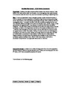
In order to prove hypothesis 4 correct I will use cumulative frequency graphs to compare the inter quartile range of boys’ and girls’ height and weight.
Having made the 4 tables with corresponding graphs I have found the results below:
This proves that the interquartile range (spread or dispersion) of the height and weight of boys is greater than the range (spread or dispersion) of the height and weight of Girls. This proves hypothesis D (which is), the range (spread or dispersion) of the height and weight of boys is greater than the range (spread or dispersion) of the height and weight of Girls) correct.
There are many possible reasons for such results and for this hypothesis to be true, however it is well known that at the age of puberty, particularly many boys tend to have growth spurts in which they grow very quickly however this may happen for some boys earlier than others and so there is a spread in the height and weight of boys, however for girls it is normally common for girls to grow around about the same time to each other which is normally later than boys and so the spread or dispersion of girls’ height and weight is relatively small, apart from anomalies such as particularly large or small girls which will obviously effect the spread and dispersion.
The next task is to use the information from the graphs to make box plots which will give an accurate representation of where the correlation is between the height and weight.
Box plots
Box plots are helpful for my investigation as they cut down data to only five numbers, the median, upper and lower quartiles, and minimum and maximum values. Also when I want to compare two or more sets of data, I can make box plots side-by-side.
The median is found by recording the data values in increasing order, and finding the central value. It divides the data into 2 equal halves, so there is about half of the data on each side.
The lower quartile is found by considering only the bottom half of the data, below the median. This means 75 per cent of the data is above this value. The upper quartile is found by considering only the top half of the data, above the median. This means 75 per cent of the data is below this value.
When you subtract the lower quartile range from the upper quartile, you get the interquartile range. This represents the middle half of the distribution 50%, and shows how far the data is spread around the median. The more spread out it is, the larger the difference between the values.
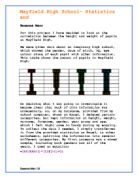
The box plots have been made using the figures from the graphs. They have been made showing height separately and weight separately. But the boys and girls box plots have been put on the same sheet to make it easier to compare the two genders.
After studying the results of the box plots it has been found that because the box plots have been made using the figures from the previous graph’s, they again confirm that the dispersion of the height and weight of boys is greater than the dispersion of the height and weight of Girls. The box plots also show that Boys’ and girls’ heights are skewed negatively, mostly spread in-between the median and lower quartile where as Boys’ and girls’ Weight is skewed positively, spread between the median and upper quartile.
These results show that (from the data which was used) most students’ height was in the lower quartile range and their weight was in the upper quartile range.
The next task is to do the scatter graphs these use the original data of the 100 students being analysed. Height is to be plotted opposite weight, So that it can be seen whether there is a positive correlation between height and weight, or not.
The scatter graphs show us that there is a positive correlation between height and weight and apart from a few inequalities height and weight of boys and girls is spread closely together. From these graph’s we can also draw a line of best fit.
The straight line comfortably fits through the data; hence a linear connection exists. The scatter around the line is quite small, so there is a strong linear relationship. The slope of the line is positive, small values of height correspond to small values of weight; large values of height correspond to large values of weight, so there is a positive correlation between height and weight. This proves hypothesis A correct.
Overall having completed the investigation it can be said that all mathematical calculations that were done to prove my hypothesis right, proved the hypothesis to be correct.
Evaluation
I feel that my investigation was accurate and worthwhile as it has told us something about my hypotheses, however I feel the investigation could have been more accurate had we also investigated and combined these results with patterns or reasons for growth in height and weight for boys and girls in years 10 and 11 (in the way we have found they do in this investigation), using other information from secondary sources such as medical or health organisations.