The total number of students is 1183. I want to select a sample of 100 students as it is approximately 10% of the total number of students and it is a suitable number for my investigation. It is suitable because it is a large enough number to give me meaningful results and should represent the population yet it is not too time consuming to handle. However, there isn't the same number of students in each year so I can't just take 20 students from each year. I will have to work out the proportion of students that I need from each year.
Year 7
(282/1183)*100= 23.8= 24 (rounded)
Year 8
(270/1183)*100= 22.8= 23 (rounded)
Year 9
(261/1183)*100= 22.1= 22 (rounded)
Year 10
(200/1183)*100= 16.9= 17 (rounded)
Year 11
(170/1183)*100= 14.3= 14 (rounded)
The following data is provided on each student:
Name, Age, Year Group, IQ, Weight, Hair colour, Eye colour, Distance from home to school, Usual method of travel to school, Number of brothers and sisters, Key stage 2 results in English, Mathematics and Science, Number of hours watched a week (average).
I will only use the following data: Year Group, Gender, Key stage 2 results and average number of hours of TV watched a week. This is because my hypothesis in that the students who watch less TV perform better.
I will use ks2 results to show the performance of the students, however, the ks2 results are given for 3 subjects: English, math and science. I will not be looking into the performance in each of the subjects; I am looking for overall performance so I will calculate the total of each of the student's ks2 results.
I also need the gender because I will split my data into gender. If I am splitting my data into gender, then I need a certain amount of boys and girls from each year. I cannot just have an equal number of boys and girls from each year because there are more girls than boys in the school. Again, I will have to work out the proportion of girls and boys that I will need in each year.
I will use Microsoft Excel to randomly select students from the list of 1183 students. I have to keep in mind that I have a specific number of students that I need to randomly select from each year. Therefore, starting from year 7, I will give a number to each student so then I have all the students numbered from 1 and 1183.
Using the RAND function in Excel I will randomly select the students. I will use the following formula to do this:
- To generate a random real number between a and b, use:
RAND()*(b-a)+a
For example, in Year 7, a is 1 and b is 278. Therefore: =RAND()*(278-1)+1
Then I create a new list with my sample of 100 students in order from year 7 to year 11.
I will present my data in scatter graphs because it shows two sets of numerical data related to each other. In this case, my scatter graph will show the ks2 results of the students against the average number of hours of TV watched a week. Scatter graphs are used to show patterns of correlation between two sets of data. A good correlation means the two sets of data are closely related to each other. A poor correlation means there is very little relationship. It would be an advantage for me if my scatter graph shows a good correlation because it would then be easier for me to prove or disprove my hypothesis. On the scatter graph I will also calculate the product moment correlation coefficient (pmcc). As I said earlier, a scatter graph shows patterns of correlation between two sets of data, pmcc shows how strong that pattern is: The product moment correlation coefficient (pmcc) can be used to tell us how strong the correlation between two variables is.
Then I will look at ks2 results to see what is affecting the results. I will make cumulative frequency tables for the ks2 results then create cumulative frequency graphs. From the cumulative frequency graphs I will be able to make box plots; these show measure of spread. To do all this I will have to calculate ranges, interquartile ranges and medians. Then, I will calculate standard deviation which shows another measure of spread. However, standard deviation shows measure of spread about the mean. The standard deviation is a statistic that tells you how tightly all the various examples are clustered around the mean in a set of data. This will help me to compare two sets of data: I this case it would be ks2 results for female students and ks2 results for male students. Then I will write a conclusion to explain to what extent my hypothesis was proved or disproved.
Sampling the Data
From the internet I retrieved the list of students from Mayfield high school. I deleted from the list the data that I don't need for my investigation. There was a total of 1183 students. I used stratified sampling to get 100 students as it is approximately 10% of the total number of students and it is a suitable number for my investigation. It is suitable because it is a large enough number to give me meaningful results and should represent the population yet it is not too time consuming to handle. I used the RAND function in excel to randomly select the students. In the plan I calculated how many girls and boys I need to randomly select from each year.
Then using excel I calculated the total of the ks2 results for each student because I need their overall performance not their results for separate subjects. On the next page, I show the list of students that I have randomly selected.
I have highlighted 4 students. At two occasions, the same student has been randomly selected twice. I haven't deleted the second time from the list because then bias would be introduced, so instead, I randomly selected 2 more students and added them to the list. Therefore, I now have a total of 102 randomly selected students.
I also highlighted an anomaly that I have spotted in the list; the student watches an average of 1,000,000 hours of TV a week. This is obvious that this is an anomaly as there are only 168 hours in a week. I will not be using this student's data for my investigation as it would greatly affect my results. Also, I would not be able to plot this anomaly on my graph as 1,000,000 is out of the scale boundaries for my graph.
Data Presentation and Analysis
Using the table in the previous pages I used excel to plot a scatter graph showing ks2 results and average number of hours of TV watched per week. On the next page the scatter graph is displayed. I also calculated the mean of average number of hours of TV watched per week and ks2 results. For both means I drew a line on the scatter graph to show it.
Ignoring the line of best fit, it appears that there is no correlation between ks2 results and average number of hours of TV watched per week. The data is equally scattered on the graph. This disproves my hypothesis, which is that the students who watch less TV perform better. Even, the student who achieved the highest results averagely watches more hours of TV per week than the mean.
However, the line of best fit drawn by the computer has a weak downhill slope; this means that there is a weak negative correlation between the two sets of data. This supports my hypothesis because a negative correlation means that the more the students watch TV the lower the results. The equation of the line shows that the slope has a weak negative gradient: y = -0.0023x + 12.328
-0.0023 means that the line has a very weak negative gradient. Therefore, this is not reliable enough to support my hypothesis. So I will split my data into gender to show more detailed results. Gender might be a possible factor that would affect ks2 results. I made two more scatter graphs, one for male and the other for female.
Now that I split my data and made two scatter graphs I see a change in results. The graph for female students shows that there is weak positive correlation between ks2 results and number of hours of TV watched per week. This disproves my hypothesis because it seems that TV does not affect the performance for female students. The gradient of the line is 0.0136. This means that the relationship between the two sets of results is very weak.
The scatter graph for male students, however, shows that there is a weak negative correlation between ks2 results and number of hours of TV watched per weak. This supports my hypothesis and the correlation is stronger as the gradient is –0.0201. The mean of ks2 results are the same for both genders. Although the girls have a higher mean for average number of hours TV watched per week than the boys, their ks2 results are not negatively affected like the boys. Although boys achieve higher marks than girls they are more negatively affected by TV than girls. The mean for the average number of hours of TV watched per week is 21 for female students and for male students it is 16.
For female students my hypothesis is disproved and for male students it is proved. I conclude that the gender is a factor that affects the ks2 results.
For each gender I will calculate the strength of correlation between the two sets of data. I will calculate the product moment correlation coefficient (pmcc). I will show how to do this for one of the genders.
Calculating pmcc for male students
The mean of the average number of hours of TV watched per week is 16, I will write this as HR. I will represent the average number of hours of TV watched per week for the students as HR.
The mean of the ks2 results is 12, I will write this as Ks2. I will represent the ks2 results for the students as Ks2.
For each student I need to subtract the mean of the ks2 results (ks2) from the student's ks2 results (Ks2); Ks2-Ks2.
I also need to subtract the mean of average number of hours of TV watched per week (HR) from the student's average number of hours of TV watched per week (HR);
HR- HR.
Sxy = ∑ [(Ks2-Ks2) (HR-HR)]
Sxx = ∑(Ks2-Ks2)2
Syy = ∑(HR-HR)2
The formula to calculate pmcc is
Then I calculated that:
Sxy = -228
Sxx = 245
Syy = 7290
Using the same method I calculated pmcc for female students.
Pmcc for female students is 0.0932 and for male students it is -0.1706. Although pmcc shows that for female students the correlation is positive and for male students it is negative, both have a very weak correlation. This means that it is possible that there is no relationship between ks2 results and average number of hours of TV watched per week. This again disproves my hypothesis.
Now I will look at the distribution of ks2 results to see how the distribution is for each gender. Calculating the range would be the simplest measure of spread, but it takes into account the extreme values. A box plot, however, excludes them and shows the Interquartile range (IQR). I made a cumulative frequency graph for each of the genders to find the interquartile ranges.
Female students- Cumulative frequency table
Male students- Cumulative frequency table
On each of the cumulative frequency graphs I drew three lines to find the lower quartile, median and upper quartile.
Male students
Lower quartile = (51+1)/4 = 13th value
Median = (51+1)/2 = 26th value
Upper quartile = [(51+1)/4]*3 = 39th value
Female students
Lower quartile = (52+1)/4 = halfway between 13th and 14th value
Median = (52+1)/2 = halfway between26th and 27th value
Upper quartile = [(52+1)/4]*3 = halfway between39th and 40th value
I then made a bigger box plot so it is easier for me to analyze.
Although the range of ks2 results is the same for both genders, the interquartile range is not. The range for both male and female students is 11. The interquartile range for male students is 3.6 and for female students it is 3. Although the boys have a higher median than the girls, their interquartile range is also higher which means that the boys are dispersed from the median while the girls are clustered around the median. This means that girls are more consistent and predictable. Whilst the boys can be very random.
I realized from my set of data that the students do not perform very well as a whole. The bar chart below shows their ks2 results.
(box plots)
Greenfield high school is another school in England but offers better education. Clearly we can see that more students in Greenfield high school achieve higher marks.
For each gender, I will calculate the standard deviation of the ks2 results. This considers deviation of a set of data about the mean. I will show how to calculate standard deviation for one of the genders.
Calculating standard deviation (s.d) of ks2 results for male students
∑f = 51
∑fx = 573
∑fx2 = 6549
The formula to calculate standard (s.d) deviation is:
Using the same method I calculated standard deviation for the female students.
For female students s.d= 1.58113883
For male student s.d= 1.483239697