Average student
Introduction
I am going to find out the year 10 male average student at Weavers School, Wellingborough, Northamptonshire in the year of 2009. I will then compare and contrast my results to the year 10 male student of the year 1996 at Weavers School. I will collect the data on hair colour, height and weight and see the differences between 2009 data and 1996 with the help of some graphs and some complex calculations
Planning grid

Sampling: Primary data 2009
I am going to collect a sample of 30 year 10 males because there are 182 students in year 10 and 94 of them are males. So 30 is roughly1/3 or 32% of the total males in year 10. 30 is small enough to be manageable and yet be representative. I am going to use random sampling method as it is not biased unlike convenient sampling. Every person has an equal chance of being selected and fairly quick unlike random stratified sampling. I will be using a calculator and the random button on the ...
This is a preview of the whole essay
Sampling: Primary data 2009
I am going to collect a sample of 30 year 10 males because there are 182 students in year 10 and 94 of them are males. So 30 is roughly1/3 or 32% of the total males in year 10. 30 is small enough to be manageable and yet be representative. I am going to use random sampling method as it is not biased unlike convenient sampling. Every person has an equal chance of being selected and fairly quick unlike random stratified sampling. I will be using a calculator and the random button on the calculator for random sampling. This is what I will be typing on the calculator:
30(Total) x Ran (random button)
Any repeats will be ignored and done again.
Secondary data: Secondary data 1996
I am going to collect a sample of 30 year 10 males because my primary data is also a sample of 30, so it will be a good comparison. Also there were 83 males in the year of 1996. 30/83 is 36% of the total no. of year 10 males which is small enough to be manageable and yet be representative. I am going to use systematic sampling because it is non biased, uses all the data and is quick unlike quota sampling which often can be biased. I will do my calculations like this:
83/30=2.7
I am going to select every 3rd student from the data and will keep going until I find 30 samples.
Pilot survey
Rules before pilot survey
- All information will be confidential and will not be shared with any 3rd party companies. There will be no names taken during the survey
- This survey will be done in a private and confidential room.
I changed the rules as I found out that students were not worried about their information being shared but had clothes and other equipment when weighing their weight and measuring their height
Rules after pilot survey
- Hair highlights will not be taken into account.
- When measuring height and weight, shoes should not be worn and should be taken off.
- No bags, extra weight should be carried when measuring the weight or when measuring the height.
- If you do not cooperate then you will be expelled for the survey.
- No outdoor coats, jumpers etc. should be worn when measuring the height and weight.
- You should stand straight when measuring the height.
- Phones, etc. should be out of the pockets and be put in a secure locker on a table next to you. Insurance will be covered for any valuables lost or damaged during this survey.
- I will do the measuring for consistency and accuracy.
Hypothesis 1
My hypothesis: I think most students in 2009 will have brown hair because most students in my class room are brown haired. I think students in 1996 will not have brown hair because my mum and dad don’t have brown hair.
My Result: I was right as most students in 2009 have brown hair but I was also wrong as most students in 1996 also have brown hair. The modal colour in both years is brown. One student in1996 had red coloured hair which is then replaced with the colour ginger in 2009. My assumption is that students now may prefer ginger as their hair colour than red. Colour blonde also has been pretty consistent as in 1996, six students had blonde hair while in 2009 five students had blonde hair.
Hypothesis 2
My hypothesis: I think most students in 2009 will be 165cm tall because I am 160cm tall and most students are a bit taller than me. I think students in 1996 will be less tall because older people who went to school in 1996 are smaller than me in height.
My result (Box and Whisker): The Tallest year 10 male in 1996 was 193cm tall while in 2009 the tallest year 10 male is 192cm tall, so I was wrong. The Inter-quartile range for 2009 was 7cm while inter quartile for 1996 was10 cm which means 1996 data was more spread out than 2009 data. 1996 data is slightly negative skew while 2009 data is slightly positive skew. There were no outliers in the 1996 data but I found 4 outliers in the 2009 data. After dealing with the outliers the range of 2009 data is less than the 1996 data which means that 2009 data is more reliable than 1996 data. I have redrawn box and whisker after finding the outliers to get a more accurate view of the spread and consistency of the data after discounting the outliers.
P.T.O
Hypothesis 3
My hypothesis: I think most students in 2009 will be 60kg as I am 50kg and most students are heavier than me. I think students in 1996 will weigh less than 60 kg as they are less tall therefore weigh less
2009
Mean (before finding outliers) = 63.9kg
∑x2=125835
Standard deviation value = 10.55 (2 d.p)
63.9 + (10.549 x 2) = 84.99 = 85kg
63.9 – (10.549 x 2) = 42.80 = 43kg
Outliers = 41kg
Mean (after finding outliers) = 64.7kg
1996
Mean (before finding outliers) = 61kg
∑x2=122651
Standard deviation value = 19.17 (2 d.p)
61 + (19.1668 x 2) = 99.3 = 99kg
61 – (19.1668 x 2) = 22.7 = 23kg
Outliers = 115kg
Mean (after finding outliers) = 59.1kg
My Result (Standard Deviation): Standard deviation value for 2009 is lower than the 1996 value which means that the weights of the students in 2009 are less spread out than the student weights in 1996. I found 1 outlier in both years.1996 data mean before the outlier was dealt was 61kg but after dealing with the outlier is 59.1kg so it is more consistent than it was. 2009 data mean before the outlier was dealt was 63.9kg but after the dealing with the outlier is 64.7kg. This means I was wrong and also means that 1996 data is more consistent than 2009 data.
My Result (Back-to-Back stem and leaf): The modal group in 1996 data was in 50-59 kg section while the modal group in 2009 is 60-69kg which means people were less heavy in the olden days. I can clearly see an outlier in 1996 section (115kg). However, that is the only outlier.
P.T.O
Hypothesis 4
My hypothesis: I think, taller the people are they are more likely to be heavier because tall people have longer bones so more weight.
My result (Scatter diagram): This scatter diagram has weak positive and also quite spread out meaning it has less consistency which is backed up by my Spearman’s rank of 0.38.This means that your weight does not depend on your height, so you don’t necessarily weight more if you are tall, so I was wrong. However, there is weak positive correlation so it also means that if you are tall you weigh more so I was also right.
Spearman’s rank value- 0.38
My result (Spearman’s rank): I was right, Spearman's rank value of 0.38 shows a mild positive correlation between weight and height which means the taller you are more you weigh. I was also quite wrong 0.38 is not a very strong value therefore inconclusive, this could have been because of different amount of fat to muscle proportion in different people.
Conclusion
Hypothesis 1: Right
Hypothesis 2: Wrong
Hypothesis 3: Wrong
Hypothesis 4: Right
So overall I was half and half, wrong and right.
The modal hair colours in both years were brown, and the least common colours were, red in 1996 and ginger in 2009.students heights are more consistent than student heights in 1996. The tallest student in 2009 was 192cm and 1996 was 193cm tall. The weights of students in 2009 are more consistent than the student weights of 1996. On average, students in 2009 weighed 64.7kg and in1996 on average students weighed 59.1kg. The taller the student is the more he/she weighs however this is not always true as the correlation is mild positive not perfect positive.
Evaluation
I have used random sampling for primary data however; I could have used stratified sampling which is fair and representative to each student in the year in different tutor groups. Also my data is only from one school so it is not very representative although this could be changed by taking data from different schools. I would do a stratified sampling for 300 secondary school form England divided into counties, there are 3000 secondary schools in England so 300 out of 3000 is 10% which is also representative. I have only done sampling for year 10 however, next time I would do sampling for all the years in school to get a better view for the average student. I have used comparative bar chart for hypothesis 1, which shows no. of people with certain hair colour. I used box and whisker for hypothesis 2 which was good as it showed me interquartile range of the two datasets and showed me outliers which helped me decide the consistency of the datasets. I used Back-to-Back stem and leaf diagram for hypothesis 3 which showed be an outlier, the range, median and the upper and the lower quartiles. I used scatter diagram and Spearman's rank in hypothesis 4 which showed me the correlation between. However, I would change some of these techniques if I were to do this again. For hypothesis 1, I would use comparative pie chart rather than comparative bar chart as a comparative pie chart shows the proportion of each hair colours in each year which makes it easier to conclude the results when compared with concluding from numbers which are read off from a bar chart. For hypothesis 3, I would use Spearman's rank which would complement standard deviation as one shows the correlation and the other will show the spread of the data, this would make a great conclusion giving me better finial conclusion.
Page of