The previous graph shows the results of the simulation which was made. The simulation was on the basis of having 1 till to be served on and 1 queue to join. As you can see that the graph shows a very wide rang of results and these results are very big. For instance some waiting times can be more than 50 seconds which is nearly a minute. This may not seem a lot but in a newsagent it is a long time.
Another factor that has come to my attenton is that the server (till tender) would be busy all the time and would have to put up with huge queues. This wouldn’t be wanted by the owner. The server utilisation is given by the following formula;
( Time server 1 busy / duration of experiment ) x 100 %.
By using my results and this formula I have found the following server utilisation:
(650 / 654) x 100 = 99.39%
This means that the server is almost certainly busy. But even though he is busy 99 % of the time customers are still needed to wait. This is because the total waiting time for all the customers comes to 1802 seconds. This is nearly 3 times as long as the whole duration of the experiment.
From all of this it is easily said that although this method is worth while, by means of server utilisation, it is still costly. This is because at the end of the day a customer is not going to wait 50 seconds at a newsagent just to buy a bar of chocolate. This would result in loss of customers and eventually might close the business down. From the simulation table it also easy to see that most of the numbers in the Waiting time coloumn are in double figures.
The newsagent that I am basing this coursework on doesn’t have just 1 till, this particular simulation was just to justify why the owner made 2 tills.
Simulation for 1 till and 1 queue.
Assumptions
- The experiment will start at time 0
- At the start there will be no customers at the till
- There are no delays in between two customers
- There will be no queue jumping
- No person leaves the queue after entering it.
Simulation for 2 tills and 1 queue.
Assumptions
- Initially no people in the queue
- No people at the till
- Time of start of experiment is 0
- No time delay between two customers
- If both tills full go to till 1 first
- No queue jumping.
Simulation for 2 tills and 2 queues.
Assumptions
- Initially no people in the queues
- No people at the tills
- Start at time 0
- No time delay between two customers
- Go to shortest queue first
- If both queues are same length go to queue 1
- No queue jumping
Simulation for 3 tills and 1 queue.
Assumptions
- Initially no people in the queue
- No people at the tills
- Start at time 0
- No time delay between two customers
- If all tills are busy go to till 1 first
- No queue jumping
The graph on the previous page shows the results of the simulation of 2 tills and 1 queue. As you can see that the graph shows a reduced range of results which are very compact. They seem to be mostly in the band of 5 seconds and 10 seconds. From the situation before, it is better as more people are served without them waiting for long periods of time. This is mainly because if one till tender is busy the other one is not so nearly all the time a till is free.
By using the results obtained in this simulation I have calculated the following server utlisation for server 1;
(383 / 679) x 100 = 56.41%
I also got the following utilisation for server 2 and by combining both of them I would get the total server utilsation.
(223 / 679) x 100 = 32.84%
And total server utilisation is 89.25%.
This states that although server 1 is busy half of the time, server 2 is not busy that much. But still this means that the customers must be getting served quite quickly. This is a good thing and is shown as an improvement to the 1 till and 1 queue situation.
The total amount of time that is waited by the customers has now dropped by nearly 2 thirds. The time for all the customers to be served comes to 644 seconds. This is a good result as it lies near the same amount of when the experiment is finished.
I can now say that this method is an improvement to the previous simulation. This is known as the waiting time is now more compact and low. The total waiting time is now at a expected value. From the table of results it is easily noticeable that the amount of double figures have been cut down and more single figure numbers are seen.
Now I am going to analyze the previous simulation that was done. It was done on the situation of 2 tills and 2 queues. As you can see from the graph that the closer you get to the end part of the experiment the waiting times decrease slowly. Although in the middle the waiting times had flickered a bit, the result is nearly the same as the 2 tills and 1 queue simulation. The only difference is that this simulation has more waiting times 4 seconds and 8 seconds. This has been a further improvement to the previous situation.
By using the results obtained in this simulation I have calculated the following server utlisation for server 1;
(355 / 701) x 100 = 50.64%
I also got the following utilisation for server 2 and by combining both of them I would get the total server utilsation.
(223 / 701) x 100 = 31.81%
And total server utilisation is 82.45%.
This is a reduction in server utilisation from the other simulations. It means that the servers are not always busy but for some if not most of the time they are free. This is because the customer workload is now shared between 2 till tenders.
The total amount of time that is waited by the customers has now dropped even more as less people are waiting more customers can be dealt with quickly and efficiently. The time for all the customers to be served comes to 623 seconds. This time will keep on going down and reducing proportional to how many tills are added.
I am able to conclude from this simulation that this is a further improvement to the waiting time but is not that affective because of the server utilisation. Server 1 is busy half of the time, which is expected but I would have thought that server 2 would also be busy half the time. This isn’t true because if both queues were the same length the customers were sent to queue 1 which had done its part.
I am now going to try to do a simulation on 3 tills and 1 queue. I think that the outcome will be that the waiting times will have been cut down but the server utilisation will again fall. This will not be the best simulation as the workers will be getting paid for doing nothing.
I am now going to analyze the simulation which has the situation of 3 tills and 1 queue. The graph clearly states that the times are more compact and have been reduced even more. This is shown in the similar results of 2 or 3 customers in quite a few places. There aren’t much values above or equal to the 10 second mark. From the table this is proved as most of the numbers in the waiting time coloumn are only one figure.
The server utilisation of this experiment comes in three different places. First of all is server 1 who I have predicted will be doing most of the work.;
(334 / 684) x 100 = 48.83%
The second place for server utilisation is server 2 who will be busy some of the time.
(180 / 684) x 100 = 26.32%.
The third and final place which server utilisation will appear is in server 3. I think he should have the least amount of work and is more or less useless.
(59 / 684) x 100 = 8.63%
the total amount of server utilisation is : 83.77%
The server utilisation of each server seperatly is very low because 3 till tenders share 1 queue worth of customers. But it surprising to find out that the total server utilisation is higher then the previous situation.
The total amount of time that is waited by the customers has now dropped even more as less people are waiting more customers can be dealt with. The total time for all the customers to be served has a total of 574 seconds. This time is lower then the end of the experiment and shows that the customers are now being dealt with very quickly.
I am sure enough to say that from this simulation it is an improvement in waiting time but in server utilisation. This is going to be the consequence of having many till tenders to customers who have small service durations.
Conclusion
I think out of all of the simulations that I have tried out the simulation that stands out and is the best in all manners is the situation of 2 tills and 2 queues.
I have come to this conclusion because this simulation and situation are best suited for the requirements of the newsagents. Since it is only a newsagents we do not too many tills as this is just useless as I found out in my last simulation. The third server (till tender) was mostly free which the owner of the shop will not like. I also found that although it doesn’t have the least waiting time it does satisfy the needs of the customer.
Below I have drawn a table to show how the total waiting time varied across all four simulations. This will give us a wider view of what was really happening.
As you can see that the waiting is always decreasing and will do so until you stop increasing the amounts of tills in the newsagent. In the comparison of the two simulations containg two tills, I have noticed that the addition of a queue has reduced the waiting time also. Since there are already two tills in the existing shop, this simulation results will be very straight forward to mark out.
Below is a table contaning the total server utilisaition which has been discussed before.
You can see that the simulation that I am justifying has the lowest utilisation. This could be for many reasons but I think the particular reason needed to explain this is that the random numbers for this simulation were not big therefore the times did not exceed the first tills limits.
I think overall my experiment was done very well and the result which has been explained above is good.