From these results I can say that the formula for the gradient is g=anx
I will see if this works for my next graphs.
…………………………………………………………………………………………..
The next graph I will look at is y=x³. See graph E.
To find out the gradient for this graph I will once again use the small increment method as I have found that it is more accurate (see calculations, page F).
When using the small increment method you don’t actually need to sketch the magnified area, you can just use the numbers and put them in the formula- (y2-y1)/(x2-x1).
I will try this when looking at the graph of y=2x³.
When x1=1, y1=2 and when x2=1.01, y2=2.060602
Increase in y= 0.060602
Increase in x= 0.01
Gradient= 0.060602
0.01
=6.0602
=6
When x1=3 y1=54 and when x2=3.01, y2=54.541802
Increase in y= 0.541802
Increase in x= 0.01
Gradient= 0.541802
0.01
=54.1082
=54
When x1=4 y1=128 and when x2=4.01, y2=128.962402
Increase in y= 0.962402
Increase in x= 0.01
Gradient= 0.962402
0.01
=96.2402
=96
I notice from the results that they are double the x³ results. I have also noticed that the results each side of 0 are the same, but the minus x’s have minus gradients. From these observations I can say that the results for 2x³ are as follows:
The graphs for x³ don’t follow my prediction of the formula from the x² graphs.
e.g. g=anx y=2x³ when x=2, g=24
but using the formula, g = 2 x 2 x 3
=12
However, the x³ graphs provide me with a new formula:-
g=anx²
To check that this formula works, I will use the final method of working out the gradient I have at my disposal, by using a graphical calculator. I will try it with the graph y=8x³. By using the graphical calculator, I produced the following table:
If I use my formula-
When x=2
8 x 3 x 2² = 96
When x=4
8 x 3 x 4² = 384
As you can see, the formula works.
………………………………………………………………………………………
I will now look at the graph y=x4. See graph F.
As using the calculator is the quickest, easiest, most economic and accurate method of finding the gradient, I will use it form now on.
For y=x4
For y=3x4
By looking at these results, I can see that neither of the past two formulas work. However, the formula that does work is g=anx³.
To prove this, I will use the graph y=3x4.
When x= -1
g= 3 x 4 x -1³ = -12
When x= 3
g= 3 x 4 x 3³ = 324
As you can see, this clearly works.
…………………………………………………………………………………………
If I look at all the formulas I have so far, I have this:
If I generalise these results, I can say that the formula for the gradient function is:
anxn-1
So if I go back to the simplest graph y=x, and add in an ‘a’ value, I can check that the formula works.
So for y=3x, when x= 4 anxn-1 = 3 x 1 x 40
= 3
As graph G shows, this is correct.
…………………………………………………………………………………………
To try and show that my formula works, I am going to explore it further, getting more complicated.
I will start with I will try y=x5. By using the graphical calculator, I get these results:
5 × 14 = 3
5 × 24 = 80
5 × 34 = 405
5 × 44 = 1280
My formula works here and so I conclude it will for any value of n.
…………………………………………………………………………………………
The equations I have tried so far all have positive whole numbers as their indices, but I want to check that this formula works on equations whose indices are negative e.g. y=x-1 and y=x-3, and whose indices are fractions e.g. y=x1/5y=x-1/2. In order to make sure, I will test out some equations.
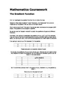
In order to make the results clear, I am just going to put the value of x, the gradient by using a calculator and the gradient by using my formula into a table.
First, I will look at the equations with negative numbers. Starting with y=x-1
As you can see the formula does work. I will still look at y=x-3 to make sure.
y=x-3
Now I will look at the equations with fractions as their indices.
y=x1/5:
This proves again that my formula works on complex equations, too. I am going to try another example to be sure. Notice that this time the ‘n’ number of the equation is a negative fraction.
y=x-1/2
If you want to work out a more complex equation such as y=4x2+3x, just divide the equation into two parts, y=4x2 and y=3x, then do it one by one as shown below:
y=4x2
y=3x
Then you combine the two together.
Using my graphical calculator I can check that my results are correct.
Just to prove that this isn’t a fluke I will do another example g=2x3+5x2 .
g=2c3
g=5x2
g=2x3+5x2
Using my graphical calculator I can check that the results are correct and they are.
……………………………………………………………………………………………………
In this piece of coursework I have shown found that you can find the gradient of any curve at any specified point for x (the gradient function) by using the formula:
anxn-1
So far in this piece of coursework I have only shown that this formula works, I have not proven it. This is what I will try to do next, I will prove that the formula works for any variation of the equation y = axn.
……………………………………………………………………………………………………
If we use a specific point on a specific line and algebra to find a gradient to begin the proof. A is the point (3,9) on the curve y=x2 (see diagram H) B is another point on the curve, which we take as (4,16). Then, as the chord AB rotates about A, B moves along the curve to B1, and nearer to A. By looking at AB as this happens, we should be able to calculate the tangent at A.
The gradient of AB = CB
AC
= CB
FG
= GB – GC
OG – OF
= 16 – 9
4 – 3
= 7
If B now moves to B1, whose co-ordinates are (3.5, 12.25),
the gradient of AB = G1B1 – G1C1
OG1 – OF
= 12.25 – 9
3.5 – 3
= 3.25
0.5
= 6.5
As we can see, the gradient is gradually becoming more accurate.
……………………………………………………………………………………………………
We can now use this method to find the gradient of another line, say y=2x2 (see diagram I), at any point. A is the point (a, 2a2), and B is another point on the curve whose x co-ordinate is a+h.
CB = GB – GC
= 2(a+h)2 - 2a2
= 2a2 + 4ah + 2h2 - 2a2
= 4ah + 2h2
FG = h
The gradient of AB is: CB = 4ah + 2h2
FG h
= 4a + 2h
As the chord rotates about A, B gets closer to A along the curve and the gradient of AB → the gradient of the tangent at A, and h → O.
As h → O the gradient of AB (2a+h) → 2a.
It follows that the gradient of the tangent at A is 4a.
So the gradient of y=2x2 at (a, 2a2) is 4a and since a is the x coordinate of the point (a, 2a2), the gradient of y=2x2 is 4x.
Just as 2x2 is where we substitute a value of x to find the corresponding y co-ordinate and plot a point on the curve, y=2x2, so we now have another expression, 4x, in which we can substitute a value of x to find the gradient at that point.
4x is called the gradient function of the curve y=2x2.
……………………………………………………………………………………………………
We can use this method to prove the gradient function for another power of x.
A is the point (a, a³) on the curve y=x³ (see diagram J). B is another point on the curve (a + h).
CB = GB – GC
= (a + h)³ - a³
= a³ + 3a²h + 3ah² + h³ - a³
= 3a²h + 3ah² + h³
AC = h
Gradient of AB = CB
AC
= 3a²h + 3ah² + h³
h
= 3a² + 3ah + h²
As B approaches A along the curve, h → O and the terms 3ah and h² each tend to zero, therefore the gradient of AB → 3a².
It follows that the gradient of y=x³ at (a, a³) is 3a², or grad x³ = 3x².
……………………………………………………………………………………………………
We have now confirmed the following:
Grad x² = 2x
Grad x³ = 3x²
The form of these suggests that the rule is multiply by the index, and reduce the index by 1; so grad x would be 5x , grad x would be 6x and so on.
So after this proof, I can once again confirm that:
Gradient of axn = anxn-1