(150 ÷ 599). 60 = 15 boys. – every 10th pupil
Since there are 150 boys in this year and 15 were required for my sample I chose every 10th pupil (150 ÷ 15). This was done for all boys and girls in all the year groups.
Year 7 Girls:
(150 ÷ 601) . 60 = 15 girls. – every 10th pupil
Year 8 Boys:
(145 ÷ 599) . 60 = 15 boys. – every 9th pupil
Year 8 Girls
(125 ÷ 601) . 60 = 12 girls. – every 10th pupil
Year 9 Boys:
(120 ÷ 599) . 60 = 12 boys. – every 10th pupil
Year 9 Girls:
(140 ÷ 601) . 60 = 14 girls. – every 10th pupil
Year 10 Boys:
(100 ÷ 599) . 60 = 10 boys. – every 10th pupil
Year 10 Girls:
(100 ÷ 601) . 60 = 10 girls. – every 10th pupil
Year 11 Boys:
(84 ÷ 599) . 60 = 8 boys. – every 10th pupil
Year 11 Girls:
(86 ÷ 601) . 60 = 9 girls. – every 9th pupil
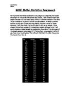
My data sample can be summarised as:
Total sample size is 120 (10% of 1200).
Method:
My hypothesis is that as the pupils increase in height they increase in weight. I have put together graphical evidence to help prove this.
To start with I shall look at year 7: to give a straight forward impression of this year I have created scatter graphs showing height against weight.
Year 7 Boys:
This plainly shows that there is a strong positive correlation of height against weight. This correlation would however be stronger had it not been for a certain ‘outlier’ (a piece of data which does not relate in proportion to the rest of the data it is with in the top left hand corner in this case). The graph following this one demonstrates my point: it is the same graph but without the outlier.
The difference is not huge but it shows that it does not take much to influence a set of data. I will not refer to this graph, though, as it is now biased – as I am fiddling the data to help fit my hypothesis better.
Year 7 Girls:
This graph is very similar to the boys of this year, with the average (the pink spot) being slightly less than the boys. The equations of the linear trend lines represent this similarity:
Boys: y = 0.0028x + 1.4347
If x is 30, y = 1.5187
Girls: y = 0.007x + 1.22
If x is 30, y = 1.43.
This strong positive correlation shown in those last two graphs is very similar throughout all the different year groups and sexes apart from two of them and I have an explanation for this. These are the two graphs:
As you can see, both graphs seem to have a slight negative correlation and particularly the year 10 boys have their data points scattered all over the place – all the points are apparently outliers.
Well, I believe this is because at these ages (years 9 to 10) children are maturing sexually and are doing this at different times, hence the unusual graph shape. It is well known and documented that girls mature generally mature sexually before boys and this appears to be demonstrated in these graphs: in year 9 it is only the girls who have a peculiar set of data points and then in year 10 it is only the boys who have a unusual set of data points.
This arouses the question: “What about the graphs showing year groups above and below these graphs?”
The answer to this is that the graphs representing the year groups above and below these ones do show a positive correlation but there are more outliers in them than the other positive correlation graphs (e.g. year 7); suggesting that these are the times when certain pupils are beginning to mature and when the rate at which they are maturing slows down.
This links up to my next hypothesis which is: “The apparent maturing of the pupils at different times affects their weight health wise (i.e. the pupils are becoming overweight or underweight during or around this period)”
To start investigating this hypothesis I have created two histograms showing “Body Mass Index” (BMI) representing all the pupils in my data sample. The group widths are boundaries of health (i.e. Underweight, Just Healthy, Healthy, Overweight, Fat and Obese) making it clearer and easier to interpret.
The first Histogram shows years 7 and 8, both boys and girls: it would be thought (regarding my previous hypothesis) that at this age the pupils would be showing initial signs in maturing. This should be reflected in the histogram by pupils either being slightly overweight due eating in excess to prepare the body for sexual maturity (this regulation of food in take is controlled by the brain subconsciously) or slightly underweight as a result of the body using up lots of fat when maturing rapidly.
Looking at the graph it is evident that there is no particular health group that is predominantly exclusive compared to the other groups apart from the “Overweight” group. What is unusual though and reflects my prediction is that there seems to a large proportion of the pupils’ information situated in the “Underweight” category as well as a similar amount in the “Just Healthy” category. This suggests that some pupils seem to be growing a lot faster than others hence are using more fat and so they are becoming tall and skinny (as I have already explained previously). In the “Healthy” category there is a similar frequency of pupils as the amount in the “Underweight” or “Just Healthy” categories which indicates that these year groups (7 and 8) are apparently under nourished. There are only very few pupils in the “Overweight” category which perhaps is what one might expect but this does not reflect my prediction. This is likely to be because the majority of the pupils in these years are not very far into the process of sexual maturing.
The second histogram shows years 9, 10 and 11. It should show more pronounced numbers of pupils in the “Underweight and “Overweight” columns – the reasons for underweight or overweight as discussed above. The quantity of pupils in these two columns is likely to be more pronounced than in the previous histogram because in these year groups (9, 10 and 11) almost all of the pupils should be maturing sexually.
Looking at the histogram it is immediately perceptible that a large proportion of the pupils represented in the histogram are either underweight or overweight more than in the previous histogram (reflecting my prediction). Only a small quantity of pupils are in situated in the “Healthy” category which is as expected and it is likely that these pupils will be in year 11 because at this age the rate of maturing is likely to be slowing down and the height and weight coming back into proportion for certain pupils.
This now returns me to my main hypothesis that the weight of the students at Mayfield increases with their height. I have previously demonstrated this relationship generally with the use of scatter graphs; I will now use cumulative frequency graphs (and box & whisker box plots) to aid with this comparison. I will only analyse cumulative frequency graphs representing year 7 girls and year 11 boys as these years are likely to be least biased and the most reliable for reasons I have already indicated (i.e. maturing sexually).
To help my comparison of these two graphs I will use standard deviation: the method with which I shall calculate the standard deviation is shown after these two graphs.
The cumulative frequency graphs are as follows:
These cumulative frequency graphs show the height and weight of year 7 girls and year 11 boys. The standard deviation (i.e. the spread) of data either side of the mean will be taken and added to either side of the mean to give two values and the mean value, these three (the third being the mean) values will then be turned into cumulative frequency by drawing a line from each one to the cumulative frequency curve and from there to the corresponding cumulative frequency values. The same will be done with the other graph and then the cumulative frequency values from each of the graphs can be compared. The more similar the results are the stronger the relationship(between height and weight).
The different year groups will be compared separately.
I have summarised the results with these tables:
It is evident, particularly in year 7 girls, that there is a correlation between the two sets of cumulative frequency values in each year group. Referring to year 7 girls, the values are very similar to each other in size and are also spaced similarly indicating a strong positive correlation between height and weight. This is due to the similar amount of points representing height and weight being accumulated going through the graphs.
Referring to year 11 Boys now, the numbers are both similar in quantity and spacing like the results for year 7 girls but not to such a degree. This can be explained by utilising one of my preceding hypotheses: that it is much more likely that there are more pupils in year 11 who are part way through puberty than in year 7 (it is unlikely that many pupils at this age are going through puberty) and therefore the correlation between height and weight will not be as strong.
Regarding the interquartile range and the median of these sets of data: both sets of graphs have interquartile ranges and medians that link to similar cumulative frequency values which again indicate the positive correlation of height against weight.
Conclusion:
I conclude generally that the taller the pupils at Mayfield High School the heavier they become.
This conclusion is firstly illustrated by the strong positive correlation between height and weight shown on the year 7 scatter graphs and the similarity between the formulas for both the year 7 trend lines supports this by suggesting that they are unlikely to be freak results – it suggests this because if there are two sets of similar data with similar correlation it is more likely that the data is accurate and worthy of taking note of.
This then lead me on to my next hypothesis regarding the affect of puberty on height and weight. The two scatter graphs which I show are clearly influenced by a certain factor which I think is due to the affect of going through puberty: I thought that a pupil is much more likely to be either underweight or overweight during this time because of excess of food in take to compensate for the initiation of puberty or the sudden use of fat for producing proteins during puberty.
To investigate this properly I drew up two histograms showing Body Mass Index (BMI) with the field boundaries representing ‘health categories’ i.e. Underweight, Just Healthy, Healthy, Overweight, Fat and Obese. These reflected my predictions positively: with more pupils being underweight or overweight than being in the healthy category. This was particularly demonstrated with the second histogram representing years 9, 10 and 11 – the peak years for puberty. This brings me to a conclusion that going through puberty does affect the pupils’ height and weight by making them become short and fat to or tall and thin; before their height and weight start to go back into proportion when they reach years 10 to 11 (hence the positive correlation returning in the scatter graphs when they reach about this age). I cannot be certain that correlation of my data is valid because I could have just got the data by chance but here is such a scatter graph to help represent this particular sub hypothesis:
This now brought me back to my original hypothesis that weight increases with height. To help demonstrate this I used some cumulative frequency graphs (four of them – height and weight for year 7 girls and height and weight for year 11 boys in connection with standard deviation: using the mean and standard deviation values for height and weight in both year groups to link them up with the appropriate cumulative frequency using the cumulative frequency curve. The results I got from this indicated a positive correlation for each year group because they were of similar value and spacing (in each year group). This is because similar amounts of data were accumulated as height and weight increased within each graph indicating the positive correlation between height and weight.
The Interquartile range also illustrates this point in a similar way.
Before I come to my final statement of conclusion it must be said that these results would have been more accurate if I had collected more data.
I finally conclude that the taller the pupils at Mayfield High School the heavier they become (but to find out whether my data produces evidence solid enough to support this conclusion, I would have to perform a statistical test).
To illustrate my conclusion generally I have produced a scatter graph with my entire data sample on it and it clearly shows that there is a strong positive correlation between the height and the weight of the pupils at Mayfield:
Evaluation:
This investigation could be improved in several different ways.
To start with: I could have made my data more accurate and reliable by choosing a bigger sample size and collecting my data sample by using random stratified sampling instead of systematic stratified sampling. This would increase the credibility of my data and hence my conclusion.
I could have made more use of different averages to support my hypothesises such as the median, interquartile range and the range (but not the mode as the data I analysed was continuous and single values are unlikely to occur more than once). More use of standard deviation appropriately would have helped as well.
To get unbiased data I used stratified sampling as this collects the correct ratio of boys to girls in a data sample compared to the original set of data. I have used a range of different diagrams to characterize my data and have also included standard deviation to increase the credibility of my data. I have also added a couple of diagrams in my conclusion to illustrate the conclusion.
Practical uses for my data could be: because my data suggests that height increases with weight generally it could be used by clothes designers to design the appropriate sized clothes.
My data could also be used for estimating the height or weight of a particular person when given only the height or weight of that person.