Example
I will press ‘shift’ then ‘ran’ on my calculator.
Say 0.088 comes up on my calculator.
I will then multiply this number by 282 giving 24.816. I will round that number to the nearest integer i.e 25
I will then select the 25th year 7 student and that student will go into my sample.
I will use the data to create scatter graphs (because they show the relationship between the two quantities) for the boys’ and girls’ I.Q versus ks points, these graphs will include the line of best fit if appropriate and the equation of a line to make further predictions. Also I will put together the boys and girls data to create one scatter graph, doing this will enable me to observe if the correlation was better when the genders were separated. Also I will be plotting cumulative frequency curves (because they enable me to get the median, upper quartile, lower quartile and inter-quartile range. This will help me to understand the spread of data about the median. I will also use histograms because I want to show that I.Q is continuous and not discrete. Histograms show the spread and the frequency density of the I.Q levels. In addition I will draw two more histograms, which represent boys and girls I.Q back to back. This will make it easier to visually compare the differences and similarities.
The data from the random selection is below
My sample
The correlation for the sample size (60) between the IQ and KS points is plotted below
The above scatter graph shows the shape of a narrow ellipse and hence show that there is a relatively strong correlation between IQ and KS results.
Positive or direct correlation is witnessed because:
- Ks increases as I.Q increases.
- Areas in the bottom right and top left are empty
- Clear linear relationship is shown
Plotted Scatter Graph for Combined Sample
The equation of a line is Y= mX + c Where m = gradient of the straight line
And c = the value of Y when X is zero.
By identifying two points on the line (from the coordinates of those two points) I was able to establish the gradient or slope of the line. The line of best fit is the best estimation of relationship between I.Q and ks points.
From the plotted combined graph the slope ‘m’= 5.1/ 17 = 0.3
The intercept of the line on the Y axis = -18.2
Therefore Y = 0.3X – 18.2
This equation can be used to make predictions of I.Q when you know the Ks value, or ks value when you know the I.Q.
From my scatter graph I can then calculate that someone who has ks points of 12 will have an I.Q of 100.7.
From my graph the I.Q value is 100 for 12 ks points. This gives an inaccuracy of 0.07.
Scatter Graphs For Boys and Girls
Both graphs show a clear tendency for the points to run from the bottom left to the top right, which indicates that a positive correlation exists between ks points and I.Q. The correlation for boys and girls from the graphs above are similar (neither show a stronger relationship than the other.) My graphs were appropriate for a line of best fit. To plot the line of best fit I found out the average of the X and Y axis and plotted the point. My line of best fit went though that point and had roughly the same number of points on either side of the line. This shows that my line of best fit is good.
Cumulative frequency investigation of IQ and KS results for combined sample of 60.
This enables to estimate the top 20% number of students having the highest IQ
Hence 80/100 x 60 = 48
So, above the point 48 on the y-axis is where the top 20% number of students having the highest IQ can be found.
If we use the cumulative frequency graph we can find the lowest grade within the top 20% of the sample by drawing a horizontal line at 48 and where it cuts the graph a vertical line downwards which represents an IQ level of 106
The cumulative frequency graph shows:
Median = 101.2
Upper quartile = 105.2
Lower quartile = 98.25
The inter quartile range = 6.95
My cumulative frequency curve is an ‘s’ shape and does not show a widely spread set of I.Q data and has a small interquartile range.
Half the students have an I.Q between 98.2 and 105.2. The data is more spread out around the median.
Histogram Analysis
The histogram for the sample of 60 shows that the distribution of I.Q levels is that what is expected for the normal distribution of I.Q readings. The back-to-back histogram for boys and girls also shows a similar distribution . The boys histogram shows a higher density at readings of 98 – 108 I.Q than that for the girls but it must be remembered that the boys sample was greater than the girls.
Conclusion
It is clear from the above that there is a strong correlation between I.Q and ks value. This has been witnessed from the scatter graphs, the cumulative frequency graph and histograms. The relationship between the I.Q and ks points for boys and girls appears from the histograms show a similar distribution. The boys’ histograms show high values between 98 and 108 I.Q levels. From the sample of girls the average I.Q value of the girls (101.71) was marginally higher than that of the boys (101.67.) From the cumulative frequency table it is possible to predict percentage ks points for students in the class knowing their I.Q values. From the combined scatter graphs it is possible to predict ks point knowing I.Q level and vice versa. The same can be determined from the individual scatter graphs from boys and girls. The results from the cumulative frequency graph and the histograms are more accurate as the calculations are derived from the frequency of occurrences of I.Q readings provided. Where as in the scatter graph the gradient is obtained from the line of best fit for passing through the I.Q values. I am happy that my conclusions are reliable because there are no anomalous results.