When I carried out the tests, I noticed some of the ways people estimated. Kerry based her estimation on 1ft to estimate 15inches. Andy used his thumb width to go along the string and estimated 42cm. Debbie guessed the length just by looking at the string, this is why her result is particularly bad in comparison to the other estimations, i.e. she did not have a sophisticated method. From the table I notice that everyone below the age of 24 uses centimeters while all those over use inches. This is very interesting as the official length of the string is 40cm or 15.7 inches. I can say that a good estimation is 1 inch or 2.5cm from the official length. Four people using inches had good estimations and four people using centimeters had good estimations. This tells me that neither is more accurate but the older you are, the more likely you are to base estimations of length on inches.
My children results read:
When I watched the teenagers estimate I found the majority just looked at the string. George measured it with his thumb as some adults had. Natalie used the end of her finger width as 1cm to estimate 31.5cm that was a poor effort. Overall, the teenagers were less accurate than the adults were; their mean is 32.37cm and the adults is 36cm, nearly 4cm difference. A good estimation is within 1 inch or 2.54cm of the official length (40cm/ 15.7 inches). Only four teenagers had a good estimation and one of those was in inches. I am going to put the results into two cumulative frequency graphs, one for adults and one for children (the graphs follow this page).
From the graph, I can see that the adult results are more widely spread, but the majority of these results are closer to the official length and the upper quartile is on that length. The median is only 2 cm away from the official length. To show how spread out those results are the box plot for adults (19cm in length) is much longer than that for children (7cm in length), this is a massive difference which shows the teenagers estimations are consistently low.
I therefore conclude that for Test 1, the adult results are more accurate than those of the teenagers are.
My second test is to estimate the weight of a bag of flour. The bag is clear plastic so they can see the flour. As an aid, I provided the estimators with a retail bag of coffee that has the weight on it so they can compare it with the flour if desired. The weight of the bag of coffee is 250 grammes and the weight of the flour is 300 grammes. I used a set of scales to weigh the flour to be accurate.
The results I got for children are:
After looking at the results of the teenagers estimations, it was interesting to see how far the majority were away from the actual weight of 300 grammes. Only three estimators were 30 grammes away from the 300 grammes, they were Jane, Gemma and Natalie. It is interesting to see that all three are girls, perhaps because they are more familiar with cookery ingredient weights. The guess that took me totally by surprise was that of Charlie, who got 1503 grammes. This is such an over estimation (it is 1203 grammes from the actual weight of 300 grammes) but she based it on cooking weights and therefore should have been a reasonably accurate estimation. Everyone compared the weight with the coffee and seemed to think the flour weighed less than the coffee, this may be down to the fact that they could not see the coffee in the bag whereas they could see the flour.
The adult results read:
It is unsuitable for me to use a mode as I had quite a few numbers with the same frequency. Although the mean is not as close to the actual weight as the teenagers one is, this is because of one of the teenage results is very high (1503 grammes) and so helped to create a closer mean. That this is the case is indicated by the adult range and median, which are both closer to the actual weight. Seven adult estimators had good results, within 30grammes of the actual weight of 300 grammes. They were Ian, Greg, Neil, Tony, Liz, Laura and Linda. Interestingly enough more males are closer than females where as in the teenage results the females were closer. This shows that as men get older they are more likely to get a better estimation than women are. Gwynne got a bad estimation because she did not use the coffee to her advantage; she did not hold the coffee and the flour in different hands like a set of scales so she was not very accurate. Neil used his hands as weighing scales and got an extremely accurate result, however no adult got the weight spot on like the teenager Gemma did.
I have produced two lots of graphs (following this page) that show the results in the table above. I notice on the adult pie chart half the results fall between 116-300 grammes whereas on the teenage one (children written at the top of the page) 55% of the results fall between 100-220 grammes. This reveals a lower set of estimates than that for the adults. On the pie and bar charts 30% of results lie between 301 and 350 for the adults. This is far closer to the actual weight than the most popular weight range for the teenagers (25% between 191-220 grammes). It is interesting to see that there are no results in the range 181-210 for adults but for the teenagers the biggest amount can be found in the two bars on their bar chart. This shows that teenagers are more likely to estimate the weight of something below its actual weight but adults are more likely to estimate the weight above but close to the actual weight.
I therefore conclude that for Test 2, the adult results are more accurate than those of the teenagers are.
Test 3 is a quantity estimation test, involving looking at a bag of conkers for a short period of time (10 seconds) and estimating the number in the bag. The bag is see-through and I do not have any specification to use the same sized conkers. I will not be letting people touch the bag to feel the conkers or to estimate the weight as this may effect their estimations. There were 23 conkers in the bag. I used 23 conkers as it was an odd number and I wanted to see if people were more likely to estimate odd or even numbers.
The adult results read:
Overall, the results are very close to the actual number of conkers. Some exceptions can be made, those being Greg who estimated badly with 50 and Kerry who also did not estimate too well with 40. I would say an accurate guess was within two conkers of the actual number present. Ten adults estimated accurately, with Hannah guessing the exact number of conkers. The majority estimated even numbers (12 estimations); this is interesting because I originally thought that people were more likely to estimate even numbers. I asked Liz why she chooses an even number and she said, “I like even numbers”.
Teenage results read:
On this test, the teenager estimations are better than the estimations of the adults. There are no ‘way-off’ results like the adults (Gregg and Kerry) but there are some very low ones, Jenny being one estimating12 conkers and Kelly estimating 6 conkers. Four estimations were made within two of the actual total making them accurate estimations: they are George, estimating the actual 23, Tim, Dan and Kate. Interestingly enough there is only one girl with a good estimation. Unlike the adults, only 10 teenagers had even. Taking the two groups together, 22 estimated an even number and 18 an odd number. I do not think these results prove that estimators are more likely to choose an even number.
I have produced two tables of standard deviation for this test and a single graph with both results on it. The standard deviation of a set of results is a measure of how far from the mean the data is spread. There are five steps in working out standard deviation, they are-
1. Find the mean of the estimations
2. Calculate the estimation minus the mean ( x – x) for each result
3. Square that difference (x-x)²
4. Multiply the total difference by the frequency (x-x)² * f
5. Take the Square root of the answer to get the standard deviation.
My standard deviation tables show that the teenagers have a smaller spread of results than those of the adults. I have also included two standard deviation to understand better the spread. Using this technique, the teenage results are so compact that 100% of their results fall within two standard deviations of the mean, while with one standard deviation, only 65% of their results can be included. The adult results more widely spread than those of the teenagers are and the results show that only 95% of their results fall within two standard deviations of the mean. The teenager mean is closer to the actual total of conkers showing that in the test teenagers are better estimators than their older counterparts are.
My final test, test 4, lets estimators use their mapping skills. I have marked on a European road map two distances from A to B and from A to C. Town A is Paris in France, town B is Biarritz also in France and town C is Rome in Italy. From Paris to Biarritz (A to B) the most direct route by road is 484miles (I calculated this using Microsoft AutoRoute Express Europe 98). I am telling the estimators this journey length and then letting them use that to aid them estimating the most direct route from A to C (Paris to Rome) in miles. I will use one large map to show the routes but these maps below show the routes and miles.
My teenage results read:
Looking at the results, I think this could be the hardest test yet as the numbers involved were much larger and the effect the directness of the roads is a complicating factor. The results look accurate with a few exceptions: Charlie estimating 1,300 miles and James also estimating 1,300 miles. I would say that an accurate estimate is within 50 miles of the correct distance of 876.1 miles. Five teenagers had accurate results: Rich, Kris, Dan, Oliver and Jenny. It appears that the females are not as accurate as the males in this test either. Three quarters of the accurate results are from males.
The adult results read:
Looking at the results they look quite a bit lower than those of the teenagers however the results are more compact in spread. The range is half the size of that of the teenagers showing a consistency in the adult estimations. Again, four estimators got good results just like the teenagers only this time it is the other way round in term of sex, 1 male and three females had good estimations. They are Tony, Ester, Debbie and Laura.
I have produced two scatter graphs using Microsoft Excel. The adult graph shows a consistency in results, as shown by the line of best fit that is almost horizontal to the line drawn through the actual distance. The best fit line is 100 miles below the actual distance (marked in on a green line).
The teenage graph shows a completely different approach to the adult graph. The line of best fit shows a negative correlation of roughly -9º. The majority of the results are below the line. I think this is because the line has to compensate for the high results estimated by Charlie and James (both estimated 1,300 miles). Quite a few results fall near the actual distance line (presented in green on the graph) but several are far below this green line. That is what makes the best-fit line form at an angle.
It is hard to decide who comes out better in this test but if I were to take the two least accurate results of each age group then the results look entirely different. The two highest results of the teenagers are the least accurate (Charlie and James’ equaling 2600 miles) and removing these reduces the mean from 805 to 750 miles. This drop demonstrates that the results are poor and the mean is distorted by two extreme estimates. For the adults, the two least accurate results are the lowest (Gwynne’s with 600 miles and Richard with 640 miles equaling 1240 miles). Their removal, improves the mean from 773 to 790 miles. Contrary to the teenager results, this shows that the two worst results adversely affected the overall results of the group. I believe this approach is valid because by using the best 90% of results, it provides a better representation of the group ability. The results show that the older you are the more likely you are to estimate a good distance on a map.
Conclusion
Looking back to the very beginning, the hypothesis was that ‘adults are more accurate estimators than children’. My results support the hypothesis. Three out of the four tests show that adults are better than teenagers are at estimating. I cannot be sure that the data I have collected is genuine as it could have been due to a small sample of data. To get results that are more reliable I could collect more data.
To find out if my data gives strong enough evidence for my conclusion, I would have to do a statistical test but having got my data and not being able to ask the estimators again it is not possible for me to do this.
One interesting observation is that in three out of four tests the teenager mean was closer to the actual measurement than that of the adults. However, by using the more sophisticated statistical analysis methods, I have demonstrated the adults to be more accurate as a group.
My results are partly from people I know and partly from people I do not know. The people I know have good educations and are from well brought up backgrounds, which could affect the way they estimate. It might make them more accurate because they have more information on how to estimate more accurately than the estimators I don’t know have a well-educated background. I could have got results that are more reliable simply by getting people in a public place on everyday of the week at different times to do my test and not to let people I know do the tests.
I made sure every part of my test was fair, I went through each test checking and re-checking that it was as it should be. I made sure no one knew any of the results and that people didn’t look on as an estimator estimated something. All my workings are double-checked and some had to be changed once I had made a second check. I made sure that my tests were fair.
My data suggests that the estimations made by adults are more accurate than the estimations made by teenagers. A practical use for this would be to employ adults that are good at estimating in a trucking firm. They could look at the speed of the trucks and the distance each truck has to travel and estimate how many trips a truck can make in a certain amount of time. That person could estimate the amount of fuel needed and how many stops the truck driver will need to take for a decent rest. A good estimator would be very useful in a job like this.