- For the third sub-hypothesis, I will use stratified sampling to get 120 data from the year 8 and 10. The final hypothesis would be shown in the form of a scatter diagram of weight against height to show the correlation between the two.
Formulas/Statistical Skills Used
Sampling
Random Sampling:
Random sampling is a method of sampling to get data in a totally unbiased way. There is a random number generator in calculator which will generate a number between 0.001-1.000. I will use the given number and multiply it by the total number of samples (population) get select the certain one that the random number generator tells. This is a good way to sample because it is unbiased so I would not have to pick each one myself.
Stratified Sample:
When selecting data from an entire population (in this case, all the students in year 8 and 10), need to know how many data I should extract from each group. I can do this by dividing the number of data in the group by the whole population’s (in this case, year 8 + year 10), we would get the ‘percentage’ of that group in that population. Then I will multiply the sample size I wish to get by the percentage. Then it would give me the number or data I need to get from the specific group.
Sub-Hypothesis 1
For my first sub-hypothesis I will use box and whisker diagrams to represent my data.
I can show the:
Upper/lower quartile, median, largest/smallest value of a sample
Median- The median basically means the middle value of the data If finding the median by hand, you need to place all the data in chronological order, then count up how many data there is. Once the total number of data is found, divide that number by 2. Then count the data from the start to the end until you reach the specific number you got by dividing total number of data by 2. That is the median, but if the sample is an even amount, then the number between the 2 numbers would be the median (e.g.: 14 15, then the median would be 14.5) evilly formulas
Upper Quartile- Found along the 75% of the data sample when the data is placed into chronological order. It is the middle between the largest value and the median of the whole data.
Lower Quartile- Found along the 25% of the data sample when the data is placed into chronological order. It is the middle between the smallest value and the median of the whole data.
Largest/Smallest Values- The largest and smallest values of the sample
Outlier seeker: There is a formula which will be very useful for me because I have box and whisker diagrams:
±1.5 x IQR (inter quartile range)
Then the number I get, I will use that positive side of it to add on to the upper quartile, then any data above that sum will be considered as an outlier. I will use the negative side of the number to add on to the lower quartile, then any data below that sum will be considered as an outlier.
Sub-Hypothesis 2
Normal distribution:
I will present the data by drawing a frequency polygon. I used frequency polygon because it would be easy for me to analyze and see whether it is normally distributed (bell shaped curve). Normal distribution is determined by many different factors such as the mode, median and mean being equal as the distribution is symmetrical, however, there will definitely be some anomalies because there are growth spurts during teenage years. I will draw 2 graphs, one will be including anomalies and one will be without any obvious anomalies. I might also use skew to analyze the data.
Skew:
A normal distribution is a bell-shaped distribution of data where the mean, median and mode all coincide (if on a frequency polygon)
If there are extreme values towards the positive end of a distribution, the distribution is said to be positively skewed. In a positively skewed distribution, the mean is greater than the mode.
A negatively skewed distribution, on the other hand, has a mean which is less than the mode because of the presence of extreme values at the negative end of the distribution.
You can calculate skew by:
Upper Quartile – Median = x
Median – Lower quartile = y
If x is equal to y, then the distribution is normal.
If x is greater than y, then the distribution is positive.
If x is smaller than y, then the distribution is negative.
Standard Deviation:
Standard Deviation is literally the mean average difference of each data item from the mean average of the entire group. It is calculated by such:
sd = square root [ ∑( x - xbar)² / (N-1) ]
Sub-Hypothesis 3
I will represent the data by drawing a scatter diagram. I will use Product Moment Correlation Coefficient (PMCC) which shows how strong the correlation is and whether it is a positive one or negative one, it refers to the line of best fit. I would have a line of best fit included in the scatter diagram. This will let me find out whether height and weight has a strong relationship between each other or a weak one.
PMCC formula:
Foreseeable Practical Problems
[Outliers]
Outliers will definitely be present because I am obtaining such a large number of data and it would give great impact on lines of best fit, distribution, and box and whisker diagrams - meaning that there would be a requirement to recognize them from the data set. When the graph is plotted, all data falling outside 1.5 of the inter-quartile range from the inter-quartile would all be considered an outlier and will be indicated in the set (for box and whisker). For scatter graph, I will try my best to spot any obvious anomalies. I will not include these in my box and whisker diagram but will plot them individually and label it outlier. I will circle outliers on my scatter graph. I will plot 2 graphs for the scatter diagram (one with anomalies and one without).
[Random Sampling]
Since random sampling is choosing data randomly, there might be a chance where it would repeat. Incase this happens, I will put a note beside the data indicating that I have already chosen it. So if the random number generator repeats a certain number which leads me to a data that I have already obtained, I will ignore it and do it again.
Analysis
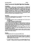
Sub-Hypothesis 1 (box and whisker diagram)
Relationship between the year groups against weight of the individual.
A sample of 60 from year 8 and 10 was collected (30 from each year group). The sample was selective so that the two genders each represents 50% of the sample for the use of sub-hypothesis 2, (although this selective random sampling may seem to be biased, it doesn’t have much affect as human population gender ration is mathematically 50:50). It was then plotted upon a box and whisker diagram in which the outliers were identified.
As you can see from the diagram - it is clear that the box and whisker diagram of year 10 is slightly to the right compared to year 8. The lower quartile, median and upper quartile has all shifted to the right by a substantial difference. The smallest and largest data value isn’t a factor in proving the hypothesis as they included outliers.
This shows that generally, Year 10’s is heavier (as on the diagram, the weights are increasing from left to right upon the axis/scale) than year 8’s. Showing that as age increases (which in this case, is classified by year groups) weight also increases due to body growth, which supports my sub-hypothesis 1.
However, although the sample themselves each represented the population in question sufficiently, the results may not be reliable as it may just be a coincidence that my sub-hypothesis was correct. Further improvements would be to investigate more year groups to show a progressive trend.
Sub-Hypothesis 2 (frequency polygon)
The weights of the genders are similarly distributed
The data of male and female are both negatively skewed (calculated by upper quartile minus median and median minus lower quartile then compare the 2 answers – formula stated above).
Male data: Upper Quartile = 60, Median = 54.5, Lower Quartile = 45
UQ – M = 5.5
M – LQ = 9.5
Therefore: UQ – M < M – LQ
Which means the distribution is negatively skewed.
Female data: Upper Quartile = 53, Median = 50, Lower Quartile = 44
UQ – M = 3
M – LQ = 6
Therefore: UQ – M < M – LQ
Which means the distribution is also negatively skewed.
But this doesn’t mean a lot, it basically only means that a lot of people are either heavier than average.
It is quite obvious that the male’s weight is slightly heavier than the female’s (the part near the end when the boys have 7 for 60kg and 4 for 72 kg). However, the difference isn’t a lot, so this means it doesn’t have a very strong impact between the relationship of gender and weight.
The mean weight for males = 55.18kg and the standard deviation = 11.24 (2 d.p.)
The mean weight for females = 50.37kg and the standard deviation = 6.73 (2 d.p.)
This shows the weight of males are slightly heavier than females (as stated above) but they are both similarly distributed – my hypothesis. The male data is more spread out but still similar to the female one, which proves my sub-hypothesis.
Sub-Hypothesis 3 (scatter diagram)
The taller the individual, the heavier s/he would be
(Please ignore the blue points on the graph, I believe it is some errors of the program so I is irrelevant to this investigation – I discovered this because these points appeared in one graph and didn’t appear in the other even when I used the same data and didn’t delete them in the other one)
For graph one, I have indicated the obvious anomalies by circling the point with pencil.
A stratified sample of 120 was collected from year 8 and 10 (69 students from year 8 and 51 from year 10). I have also used random sampling so that all biased will be eliminated. It was then plotted on a scatter diagram.
As you can see from the graph, it is clearly that there is a correlation between height and weight, however, it isn’t a very strong one. Using PMCC, I have found out that the data (without anomalies) is only 0.3965 which is near zero correlation. Although it is very near zero correlation, it is also partly a positive correlation. This proves that height and weight has a relation, but a weak one, which supports my sub-hypothesis to some extent.
However, this isn’t reliable because I only obtained data from 2 years, and it might all just be a coincidence that I got data that shows a slight relation with each other. To improve this, I might need to obtain more data throughout the school including year 7, 8, 9, 10 and 11.
Overall
From all the evidence I got:
- There is a relationship between year group and weight – seen by the box and whisker diagram shifting to the right.
- The gender doesn’t have a lot of effect on weight, just that male is slightly heavier than girls (averagely).
- Height and weight does have a relationship, but only a small one.
I can conclude that the year group has a strong effect on weight, therefore my main hypothesis is correct.
Evaluation
Overall, I think I carried out this data handling project to my greatest ability. However, there are a few obstacles which I encountered. At the start I sampled a lot of data from year 7 – 11. I also made some sub-hypothesis that wasn’t very good for contributing evidence towards my main hypothesis such as: The distance traveled by a student and their weight. This wouldn’t work because what if they rode a bus? What if they rode a car? Therefore I wasted a lot of time on collecting data that in the end I didn’t need or use. My planning was pretty good in my opinion, but the wordings I used might not be the best and probably didn’t convey the message to the examiner very well. If I didn’t waste the time on collecting the data that I didn’t need, I could have made a lot of improvements for my project. Improvements such as: increasing the range and taking samples from the whole school, which could show a progressive trend for my first sub-hypothesis (main hypothesis). I could also use my time more effectively by studying some other high level statistics formula that may be very useful for this project. This would allow me to use more skills throughout the project. Finally, I am not sure whether I made the right choice to draw a frequency polygon instead of a histogram, I could have consulted the teacher about this problem earlier to make sure the quality of this project is at the
Extensions could be made to my handling project. Although I have already included a lot of information that is sufficient to support my main hypothesis, it might not be a very reliable way. If I could extend, I would increase the range of year groups I use (as stated above), I will use the whole school. This might give another effect on my hypothesis. Since the range is so small, my hypothesis is correct but if I took a larger range of data, my hypothesis might be incorrect.
Some other hypothesizes that I might investigate on:
- Relationship between what transport they ride and weight (to see whether most of the people with light weight do more exercise – walking/bike) However this might be limited to people who are near the school because what if students live very far away, it is not possible for them to actually walk to school or ride a bike. (if I wanted to investigate on weight again)
- Relationship between height and their favourite sport (to see if there are certain sports that can boost their height because some sports like cross-country wouldn’t)
- Relationship between year group and their IQ (since I already found a relationship between weight and year group, I will use this chance to find more relationship that might exists between year group and other things)
- Relationship between weight and average number of hours watching TV (to see whether relatively heavier student spend more time watching TV, which might cause lack of exercise)
These questions will let me gain more understanding on relationship between our body and how what we do in our lives.