From this graph, we can conclude the following:
- As the mileage of a car increases, its price decreases.
- As the mileage of a car increases, it becomes more and more dominated variable for estimating its price.
- For cars with small mileages, their prices vary very much by other variables, such as the brand or engine size. Where as for cars with low mileages, their prices largely depend on their mileages. Same situation as the one in the graph, relationships between the Price and the Age.
3. From these two graphs above, I can conclude that since age and the mileage show similar graphs. This tells us that they are both linked. And this is obvious because they both show the same pattern of the line in both graphs. I will plot a graph showing the link between the two variables that are the age and the mileage and it is shown in the next graph.
This graph shows me that the age and the mileage are very closely linked. The gradient of the best-fit line is close to 10000, which means it shows that the link is very close to 10000 miles per year. The y-intercept should show 0 in theory because the car was not driven when it was new, but in this graph, it shows that the y-intercept is 4435. This tells us that there’s an error on this graph. The value r on the graph is close to 1, which means a very strong relationship between these two variables. Again, there is a problem on this graph, because a point (circled in red) seems to be out of place again. This car is exactly the same one as the one on the previous graph. This car has been used more frequently than the others and its mileage is much higher than the other cars.
The conclusion for this graph is:
- The age of a car is directly proportional to its mileage.
- The average mileage per year is 10563 miles/year.
4. I think that the engine size might have a relationship with the price of the car, because as a bigger engine might wear out quicker or be more expensive. However, it doesn’t show a great relationship and importance on the actual price, according to the graph shown below.
This graph clearly shows us that there is no correlation here in this graph between the Engine Size and the Price. The trend shows us that the bigger the engine size, the higher the price. But the relationship is very weak. Although there are 2 cars with the same engine size, the price difference is very big.
From this graph, we can conclude that:
- The Engine Sizes has no links between the Prices of the cars.
5. Previously, I did a graph on the relationship between the price and the engine size and the correlation came out not very strong. So this time I am going to bring in the Original price instead with the Engine size to see whether these two variables will have some sort of relationships.
I was surprised to get this kind of result from these two variables. Previously we had tried the graph with the Price and the Engine Size and it did not come out very well because there was no correlation, but this graph shows a strong correlation. This means both of the variables are closely linked. The y-intercept for this graph should show a positive value, because the car without the engine must cost something, but the value comes out as negative, which means there’s an error. From this, the conclusion can be made which are
- The original price of a car is directly proportional to its engine size.
- For every increase of one litre of the car’s engine size, its price increases 7528 pounds in average.
6. I think there will be a quite a strong link between the Original Price and the Price (Current price), because the higher the original price is, the higher the car price would be if the other variables don’t play a part in this. But sadly other variables do play a part in this. But I will plot it anyway to see whether it has an affect or not.
From the graph, we can see that the relationship between the Price and the Original Price is not very strong. One originally expensive car has very low price, as shown on the graph (Red circled). This car could have been affected because it could have been influenced by other variables such as the brand of the car. When the car was bought, the brand of the car was well known, but when it came to selling the car, the brand might have been considered as not good any more like in the old days.
From the graph, these conclusions can be made:
- Not a great correlation can be made from the Price and the Original Price. This means they are not linked very strongly but are linked in some ways.
Now that I have found the links between the data that I have and the current price of the car, I can process the data logically to form better conclusions. From the data given, I will try to see if there is a constant price decrease where
Decrease = Original Price – Current Price
As you can see above on the graph, the points are all over the place. I would say that there is not correlation here on this graph. I believe there is just one problem in this table. This table shows the price decrease where the Original Cost subtracted the Price (Current Price). But there is no constant decrease, because the age factor has not been worked out onto the table. Some cars have higher age than the others so therefore I must divide the Price decrease with the Age (Year). The next table will include the Price decrease divided by the Age (Year), which will tell me the price drop per year.
These results will still not show a good correlation between the Price decrease per Year and the Price. As you can see on the graph, the correlation is still not good enough. So there must be another variable, which have an effect on this. I believe the Engine Size and the Brand (Make) of the cars will affect the rate. Prices may drop as some brands are more popular than others and therefore the Price will decrease at a slower rate. Engine with a large size might wear out slower or faster meaning the rate of decrease (Price decrease per year) will also be affected. I will first plot the Price Decrease per Year against the Engine Size, and then the Average Decrease per Year against the Make (Brand) of the cars.
By looking at the graph above, I can see that there is no correlation between the Price decrease per Year and the Engine Size. So I think the Engine size won’t matter that much and won’t affect a lot in the Price.
And I think there will also be no correlation between the Price decrease per Year of the each brands’ cars and the Price (Current Price). Here is the graph:
As I have said above, I think I am correct. This graph also shows me that there are some kind of relationships between the brands’ price and the decrease per year. But it seems as though only Ford, Peugeot, Vauxhall and Rover’s trends go positive but Fiat is the only one, which is going negative. Still one brand (Fiat) is an odd one out which means it still can’t be said to be a major influence.
From these two graphs shown previously, I can therefore conclude that I can never find a specific value of the price and the value will be changed depending on the variables that affect it. Using what I have done so far such as graphs and the data, I will try to find a formula (Model), which can accurately identify the price of the cars.
Percentage Decrease:
Decrease means how fast the cars depreciate (decrease in value). If we Original Price – Price, we will find the actual money which was depreciated. But if we want to find the percentage depreciation, we must use this equation: . This has been built up from year to year since the beginning when the car had been bought. Since each year the car’s price is less, this decrease is in a different initial value each year, which leads to a compound decrease (Depreciation rate).
Creating a Model:
Now I will attempt to find a model using my knowledge and the data, which I have done so far. I’ll first make the Price as the subject of the formula, because this formula is to work out the price. This is called a compound interest model that is used in banks to calculate the people’s interests.
Now, I need to come up with a formula (model function) that will show the ‘product moment correlation coefficient’, which will decide whether it is a perfect positive/negative relationship. To find the formula for the depreciation rate, I need to draw graphs, and etc and then come up with some ideas for the formula.
First of all, the price must never come out as a negative value or should never reach 0, so the rate of depreciation has to be bigger than 0 but smaller than 1. It can be shown as like this:
This is because it is a rate of price decrease per year that means it can never be over 1 but has to be bigger than 0. So it can be expressed as:
- P = Price
- OP = Original Price
- R = Rate of Depreciation
- Y = Years
We can use this model for now for the depreciation of cars, as it is similar to compound interest, where the cars depreciate a percentage every year. As the year goes up, the price must also go down. If we make the R as the subject of the formula, it can come out as like this:
R is not a constant of any kind. R can never be constant. R just indicates the percentage, which a car has depreciated since the previous year. R is actually very complicated function, which contains many different variables.
If the equation of the graph was y= -0,0055x+ 0,2191 and I changed it into an equation which was subject to the rate of depreciation. And the equation came out like this:
R= -0,0055T+ 0,2191
Y-intercept for this graph is: 0.2191 and the X-intercept is: -0.2191/-0.0055 = 39.8
By using this formula, I substituted the R from the formula with the equation and at last in the end, the formula worked like this:
I substituted the equation of the linear graph with the rate of depreciation, because this equation from the graph represented the rate of depreciation in an equation. I believed by replacing the R from the model that is similar to the compound interest model, which contains numbers and a variable, I believed I could find out the present price of the cars.
From the graph below, I can see that as the age increases, % depreciation rate decreases. This means that as the age increase, the depreciation is getting slower and slower. The gradient of the curve at any point is a measure of how fast cars depreciate. The y-intercept on this graph means the original depreciation. It is the depreciation when a car has been bought. This graph tells that the average original depreciation is 21.9%.
Experimenting the Model:
In this investigation, we are trying to find out a way to predict a car’s price after a period of time, which is in years. This is based on variables, and for this investigation, there is no right or wrong model. But there is a possibility that one model can be more accurate than the others. Theoretically, more accurate model could be much more complicated than the less accurate model. More complicated model could include more variables, longer calculations, more time will be needed in order to be much more efficient.
Based on these facts and considerations, I have decided to use a model, which is very similar to a compound interest model:.
In this model, the only unspecified variable is R, which is the rate of depreciation. Therefore it is very important to be able to predict the value of R based on given variables. The main task of this investigation is to find a suitable model for R. Once that is done, the price of the car can then be easily estimated from that model. I decided to use Age to predict the value of R, because it affects the Price the most.
In other words, I will make a graph of each of the cars’ brands. To that, we leave the variable less for the brands. The graph will be the rate of depreciation against the age. Then I will plot a trend line that is linear and then I will find out the equation of that linear graph and then substitute it with the rate of depreciation, which is R. The graphs are shown below:
So the Model for all the brands can be written down like these:
Fiat:
Ford:
Peugeot:
Rover:
Vauxhall:
A model for depreciation rate can be created this way:
- G = Gradient of the trend.
- I = y-intercept of the trend.
All the different brands of the cars have different values.
So, for example, if the trend (correlation) had 0.34 for the gradient and 0.124 for the y-intercept, it can be converted into the following way:
By using this model, you can predict the price easily and the price is quite close to the real price. But most of the predicted prices have some errors of ±500 pounds.
Now, I will attempt to make a graph where the calculated price (calculated by using the modal) against the current price. By doing this, I will be able to see whether the modal is accurate or not and evaluate it. At first, I will do the graph on the calculated price for all the brands, and then I will go on to each of the brands. If I find out that the results are not good enough, then I will be able to change some parts of the equation to make it much better.
All Brands:
Fiat:
Ford:
Peugeot:
Rover:
Vauxhall:
By looking at these graphs, I can conclude that the calculated results are very accurate indeed. Because each graph shows us there is a linear relationships between the calculated price and the current price. Even though the trend is not plotted for all the graphs, I think the regression squared value (a value between –1 and 1 which shows how strong the correlation is, with 0 being the worst and –1 and 1 being the strongest negative and positive correlation respectively, which indicates how good the relationships are. The regression-squared value is not shown in the graph, but it is definitely very near to 1, because of just simply looking at the graphs. Therefore I will conclude that the modal was a success for each brand and also the one that was the average for all the brands.
Conclusions:
Here is what I have found out in this investigation about the selling used cars and is done in bullet points:
- Very good correlation between the age of the cars and its mileage, which means that the age is directly proportional to the car’s mileage.
- An average car travels at 10563 miles/year if mileage have travelled an average number of miles
- The age and the mileage are similar and will not make a lot of difference when using either of them when trying to find out the present price of cars.
- A good correlation between the mileage and the price
- The price decreases as the mileage increases
- The price decreases as the age increases
- A good correlation between the cost of the car when new and the engine size
- As the engine size increases, the cost of the car when it is new also increases direct proportionally
- The average increase in the cost of the cars is around 7528 pounds per every litre of engine size
- No strong correlation at all between the present price and the engine size
- There is no correlation between the decrease in the price of the car per year and the engine size
- The engine size does not affect the depreciation of the cars much more than the other variables
- For some of the cars, engine size affect the price a lot and for some other cars, the engine size does not affect the price a lot
- There is no constant decrease when the decrease in price is divided by how old the car is
- The model function is similar to the compound interest model but decreasing
- The rate of depreciation is not constant, because it is affected by many other variables, such as the age and the original price of the car, and also the current price of the car, mileage and also the engine size
- Depreciation rate of a car indicates just how much the price of a car depreciated (in %) since the previous year
- The depreciation rate of cars slows down as the age/mileage increases
- I predicted present price becomes more accurate if you separate the model formula into each of the makes
- You can replace the equation from the linear line (best fit line) of the depreciation rate and the age with the depreciation rate from the model formula to make the depreciation rate constant (it is in numbers) and to calculate the current price
- The brand Fiat is the cheapest from the rest of the brands
- Fiat car is quite cheap due to a lot of variation in the size of the engine
- Rover and Vauxhall are technically more expensive than the other brands
- Ford have the most expensive cars when it is new
- Ford tends to have the biggest engine size than the rest of the brands
- All Peugeot cars have the smallest engine size than the rest of the brands, and that is why it makes them the cheapest cars when it is new
- The brands have quite a big impact on the model formulae, and therefore each model formula has to be made for each brands to make the predicted price as near as possible to the real present price
-
The average formula for all the brands is: . This is true, since the gradient and the y-intercept were taken from the graph where the rate of depreciation was against the age. On this particular graph, it was not done with each brand and contained all the brands.
- The model formulae that is used to each of the brands are as follows:
Fiat:
Ford:
Peugeot:
Rover:
Vauxhall:
-
Each specifically specified model for each brands are much more accurate than the model which is the average formula for all the brands. The average formula for all the brands has the error of around ±1000, where as the each brand’s formulae has ±500 pounds of error. So I could conclude that each brands’ model is much more accurate.
- So it is the best to use the model function formula for each brand to get the most accurate results. But the predicted price may come out slightly faulty, but it would still be much more accurate than using the universal formula for all of the brands.