In total, I sampled 50 and each year group was stratified to provide me with a signified number of samples which is from years 7 to 11, boys and girls. This will now allow me to create complex graphs to present the data to enable me to spot any trends, relationships or anomalies in the data for height, weight, year groups, age and gender.
I will present all the averages and totals for the boys’ and girls’ means, modes, medians, ranges, quartiles and deviations into tables and charts so that I can look at it anytime in which I will attempt to interpret and conclude from.
From the data that I have collected above, I can see that there are two incorrect data values because there is a girl that weight 110kg and a boy which weighs 9kg.
This is obviously very extreme, but I think that if I don’t keep these points, it won’t make the investigation entirely fair because I would have to choose another person which would make the data somewhat biased. So therefore, I have chosen to keep the incorrect data to mention this human error in my anaylsing of the graphs.
Outliers:
Outliers are extreme values in data sets and are often ignored as they can distort the data analysis. We make the concept precise by defining an outlier as ‘any value which is either 1.5 times the inter-quartile range (IQR) more than the upper quartile (UQ) or 1.5 times the IQR less than the lower quartile (LQ). Any outlier should be marked on the box and whisker diagram but the whisker should extend only to the lowest and highest values that are not outliers.
Product-Moment correlation coefficient (PMCC)
The product moment correlation coefficient (PMCC) can be used to tell me how strong the correlation between two variables is. A positive value indicates a positive correlation and the higher the value, the stronger the correlation. Similarly, a negative value indicates a negative correlation and the lower the value the stronger the correlation.
If there is a perfect positive correlation (in other words the points all lie on a straight line that goes up from left to right), then r = 1.
If there is a perfect negative correlation, then r = -1.
If there is no correlation, then r = 0. r would also be equal to zero if the variables were related in a non-linear way. This is the formula for product-moment correlation coefficient:
r = SUM((x-xbar) (y-ybar)) / SqRoot [SUM((x-xbar)2(y-ybar)2)]
√∑(x-) (y-)
√(x-) ^2(y-) ^2
Data Presentation and Interpretation
The yellow lines on each scatter graph are constructed to indicate to me what the mean height and the mean weight of the data, thus, providing me with information on what the average height and weight should be for a boy or girl in each year.
Here is a scatter graph which shows the heights and weights for everyone in my sample of 50.
This graph is very significant to provide me with enough data to prove or disprove one of my hypotheses, ‘as the height increases, the weight also increases.’ I drew a line of best fit to show me this correlation. There are a few anomalies in the graph, however the two mean lines for the height and weight indicates me the average point of both variables. Most of the points are clustered in that area which tells me that most of the points is around that mean average. I can spot a positive correlation by looking at the number of points in each quadrant. If the points are mostly in the bottom left and top right, the graph is positive. If most of the points are in the top left and bottom right, this will be negative. The yellow lines help me to indicate this. If the points are about the same everywhere and scattered anywhere, this can be considered as no correlation.
The points on this graph are more frequently spotted in the bottom left and top right quadrant indicating me that this is a relatively weak positive correlation. I will use product-moment correlation coefficient to find out how strong the positive correlation is between the variable for all the boys and girls.
Here is the PMCC table which calculates all the boys and girls from my sample (50).
With this result for the correlation for all the boys and girls in the sample, I have gathered that there is a relatively positive correlation because it is about the middle between 0 and 1 which is neither a no correlation nor a very strong correlation. I have to consider that there are a couple anomalies which could have possibly distorted the means which could in turn alter the PMCC for the whole of the high school.
This graph and calculations have aided me to conclude on my hypothesis including ‘as the height increases, the weight increases.’ This is a basic hypothesis which can be proved by using this scatter graph which clearly illustrates the relationship between the two variables.
This is a scatter graph displaying the heights and weights for all the boys.
There is a definite correlation for these variables; however, there are a few anomalies which are probably mistakes which happened when entering the data. Since product-moment correlation coefficient allows me to view how much this set of data is positive or negative, I will use this to see how positive the relationship is between the variables.
There is a relatively strong positive correlation for all the boys. From the line of best fit, I can see that there is a positive relationship, but with the PMCC, I can certainly see that there is a positive one.
Below is a scatter graph which shows the relationship between the height and weight for all the girls.
I can easily see that there is a large positive correlation just from observing the line of best fit. There is one anomaly, but this doesn’t distort the means. From the bisecting lines, I can see that most of the points for the girls are surrounding that equilibrium.
The girls are almost the same as the boys because there is a line of best fit which indicates there is a positive relationship. With the result from the PMCC, I can see that there is a relatively strong correlation but still not as much as the boys.
This is a scatter graph which shows the correlation between the age and height for the students in the sample.
This is a graph displaying the ages of all the students in the high school sample which corresponds to their height. The mean for the height is 1.61 m and from this line, I can see that most of the points lie on this line. This shows that besides the age, the most common heights are around 1.60. As the age increases, the number of points above the line increases, which demonstrates that as people grow, they grow taller. For instance, there is a large number of peoples’ heights that are below the average at age 12, but at age 16, there are no heights under the mean. This clearly proves my hypothesis true about as the person grows older, their height increases. I can see from this graph that this statement is true. For example, the tallest height for a 12 year old was 1.80 m, but the tallest height for a 16 year old was approximately 2.05 m. This clearly indicates that there is a positive relationship; as the age increases, the height increases.
I have calculated standard deviations for boys and girls. The standard deviation is a measure of how spread out your data is. Computation of the standard deviation is a bit tedious. The steps are:
- Compute the mean for the data set.
- Compute the deviation by subtracting the mean from each value.
- Square each individual deviation.
- Add up the squared deviations.
- Divide by one less than the sample size.
- Take the square root.
These are the standard deviations for the boys and girls.
The standard deviation for the boys is much bigger than the girls. This is because the boys’ data is more spread and the range is much larger. The girls’ data is all about the same with a few low and big heights. The deviation is very low and the range is lower than the boys which indicates to me that most of the girls’ heights are all around the mean and are all about the same.
I haven’t done any calculations for the weights for the students because it is not relevant to what I am interpreting to help me answer my hypotheses. The only hypothesis that is relevant to weights of students is ‘as the height increases, the weight increases.’ This has already been displayed in a scatter graph showing that all the boys’ and girls’ heights and weights. So therefore, the next few calculations and averages are relevant to comparing the heights for the boys and girls to answer my other hypothesis, ‘boys have a higher average height than girls.’
In my plan, I have stated that I will create stem and leaf plots to calculate the main averages for the data including the boys, girls and both.
Here is the stem and leaf plot which shows all the heights from the sample.
Key: for example: stem 1.3| 2 = 1.32 metres
They are all in order from least to greatest for each stem because this will allow me to calculate the median height.
Here are the series of calculations which was helped by using the above plot.
Mean = sum of all heights ÷ total number of students
= 1.61 m
I have rounded this to 2 decimal places because this is a good degree of accuracy.
Median (50 percentile for the data)
= 50 ÷ 100 × 50
= 25th value
= 1.60 m
Mode (most occurring value)
= 1.65 m
Range (highest value lowest value)
=0.75 m
Upper Quartile (75 percentile for the data)
= 75 ÷ 100 × 50(total number of students)
= 37.5th value of the data
= 1.665 = 1.67 m
Lower Quartile (25 percentile for the data)
= 25 ÷ 100 × 50
= 12.5th value of the data
= 1.52 m
Inter Quartile Range (Upper Quartile Lower Quartile)
= 1.665 1.52
= 0.145 = 0.15 m
Now I will do two other separate stem and leaf plots for the boys’ and girls’ heights which will allow me to calculate the averages to help me compare the average height for the boys’ against the girls’.
Here is the plot for the boys’ heights.
Key: for example: 1.3 | 2 = 1.32 metres
Here are the series of calculations for the averages that I need to answer my hypothesis. I will use the same exact formulas for the mean, mode, median, range, inter-quartile range, upper quartile and lower quartile as I calculated above with the previous stem and leaf plot (both boys’ and girls’ heights).
Mean = 1.63 m
Mode = 1.65 m
Median = 1.61 m
Range = 0.74 m
Upper Quartile = 1.6675 = 1.67 m
Lower Quartile = 1.5575 = 1.56m
Inter-Quartile Range = 1.67 – 1.56 = 0.11 m
Here is the plot for the girls’ heights.
Key: for example: 1.3 | 0 = 1.30 metres
Here are the calculations for the girls’ heights.
Mean = 1.59 m
Mode = 1.6 & 1.5 m
Median = 1.595 = 1.60 m
Range = 0.49 m
Upper Quartile = 1.6575 = 1.66 m
Lower Quartile = 1.505 = 1.51 m
Inter-Quartile Range = 1.66 – 1.51 = 0.15 m
Here is an organised summary of the results I calculated by using the stem and leaf plot.
For all the calculations, I rounded the answers to two decimal places because I think this is an accurate degree of accuracy and easy to interpret from if the result has less numbers.
My hypothesis is that boys have a larger average height than girls. From the calculations I can see that this is true. The average height for the boys is 1.63m and the girls’ average height is 1.59m. This is a difference of 4cm which is quite large for an average. The most occurring height for the boys was 1.65m and for the girls it was 1.6 and 1.5m which indicates to me that there are more boys that are taller than girls. The median however, is almost the same which back slaps that last statement. The median is the 5oth percentile of the data and from this, the median tells me that perhaps that there are many heights for the girls that are around 1.6m. For the boys, this could just be a random average value that wasn’t very common and it was in the middle. The range clarifies that the boys’ heights have a wider spread of data which means that there are more heights that are taller. The girls’ range was really much smaller compared to the boys which indicates to me that the girls’ heights are all about the same as the mean. The upper and lower quartiles and the inter-quartile range are used to help me to construct a box and whisker plot to compare the boys’ and girls’ heights. Also, the column for both (everyone) helps me compare the averages for the girls and boys to the entire samples’ averages.
The mean for the whole sample was 1.61m; the boys are 2cm more and the girls are 2 cm less. This also concludes the fact that the boys’ average height is more than the girls. The range for the whole sample is almost the same as the boys which indicates to me that the spread of data for the whole sample is about the same as the boys spread. The inter-quartile is exactly the same for the girls’ and the total for both which says the opposite of what the range told me. The inter-quartile range is the difference between the upper and lower quartiles which also tells me the spread of data. The upper and lower quartiles are almost the same which indicates to me that there is a similar spread of data. This brings to the conclusion of constructing a box and whisker to clarify that statement.
This is a box and whisker plot showing the boxes for the boys, girls and both/mixed.
If I compare the boxes for the girls’ heights and the boys’ heights I can see that the boys’ box is much smaller than the girls’ one. This indicates to me that the inter-quartile range is smaller also. The box and whisker diagram shows that the girls’ inter-quartile range is 4cm more than the boys. This suggests that the boys’ heights are less spread out but they are more compressed at a higher median. This is puzzling because from my standard deviations that I calculated previously, it evidently shows me that the boys’ deviation was much larger than that of the girls indicating me that the boys’ data is more spread out or skewed. However, the length of the box in the diagram shows differently. Since the standard deviation is more accurate and reliable, I will use that instead of the inter-quartile range given in the box and whisker plot. The lower quartile for the boys is 5cm more than the girls suggesting that there are more boys with increasing heights than that of the girls. The whiskers spread much more because the highest value for the boys is 2.06m and the highest for the girls is only 1.80m giving smaller whiskers or less skew. Since the boys’ whisker stretches very far, this implies that this is value is an outcast which is causing skew. So therefore, I will deduct the length of the whiskers to make sure that any value which is either 1.5 times the inter-quartile range (IQR) more than the upper quartile (UQ) or 1.5 times the IQR less than the lower quartile (LQ). Any outlier is marked on the box and whisker diagram but the whisker extends only to the lowest and highest values that are not outliers. Once I have all the outliers calculated, I will make amendments to the above box and whisker plot for the boys and girls.
Boys
Upper Outlier = 1.5 × IQR (0.11) + upper quartile (1.67m)
= 0.165 +1.67m
=1.835m
Anything above that value is an outlier which I will then only extend the whiskers to the highest value under the upper outlier (1.835m).
Lower Outlier = lower quartile (1.56m) - 1.5 × IQR (0.11)
= 1.56 – 0.165
= 1.395m
Anything lower that value is an outlier which I will then only extend the whiskers to the lowest value above the lower outlier (1.395m).
Girls
Upper Outlier = 1.5 × IQR (0.15) + upper quartile (1.66m)
= 0.225 + 1.66m
= 1.885m
Anything above that value is an outlier which I will then only extend the whiskers to the highest value under the upper outlier (1.885m).
Lower Outlier = lower quartile (1.51m) – 1.5 × IQR (0.15)
= 1.51 – 0.225
= 1.285m
Anything lower that value is an outlier which I will then only extend the whiskers to the lowest value above the lower outlier (1.285m).
I have noticed after the calculations involved above, that there are no outliers for the girls, however, there were outliers for the boys. This indicates to me that there is a wider spread of different heights, both low and high. The whiskers now are more closer to the box then before which indicates to me that most of the heights are in the boundary from 1.47m – 1.80m; this is actually a large range of heights (boys have a large spread of data). If I look at the girls, I can see that the heights extend lower than the boys lowest outlier so therefore, most of the heights for the girls are in the boundary from 1.31m – 1.80m.
Conclusions
Investigation
The start of the investigation was to choose a line of enquiry and hypotheses to prove or disprove using statistical calculations and graphs to help to interpret from to conclude the hypotheses. I then collected the data; I chose 50 samples out of the 1183 because I thought it was big enough to reflect the population. To sample, I first used stratified sampling to split the year groups into boys and girls. After I knew the amount from each year I needed, I used a random number generator that chose random students which would provide a way of sampling that wasn’t bias. After I had all the data, I presented the data into scatter graphs, tables box and whisker plots which provided me with information to conclude on the data. From each presentational method, I interpreted to help me make an educated conclusion to prove or disprove the hypotheses. Lastly, after I have all the conclusions for each graph, table or diagram, I now have to relate it back to the original hypotheses in my plan, which is what I am doing below (subheading: conclusions on hypotheses).
Conclusions on Hypotheses:
- As the height increases, the weight increases
From the scatter graph that displays the height and weights of all the 50 students I sampled, I can see that there is a positive correlation. So this graph was very reliable and very resourceful because it evidently presented that as the height of the student increases, the weight increases also. To make up that correlation with a more accurate calculation, I used PMCC which exactly told me that there was a relatively strong positive correlation which was about half between 0 and 1 (1 being perfect positive and 0 being no correlation). Even though it wasn’t exactly a really strong positive correlation, it still proved that as the height increases, the weight increases also. If I had more time, I would have presented this data in other various graphs and charts which would help me give me a more accurate understanding of the variables and the relationship that is evident.
- As the age increases, the height increases
This hypothesis was another easy one to prove or disprove because of the scatter graph I created. This graph enables me to see the link between the age of a person and their height. The graph evidently showed that as the age increases, the height of the person increases also. There were no real other graphs or charts that I could do to prove or disprove this hypothesis so this is why I chose to use a scatter graph to present the data for further analysis. I am not sure if any other presentational methods are suitable or relevant to this hypothesis so this is why I didn’t do any other.
- Boys have a higher average height than girls
This hypothesis has been proved due to the box and whisker plot showing the median for the boys’ and girls’ heights and all the calculations that I have done to show this relationship. The girls’ median height is 1.60m and the boys’ median height is 1.61m; this shows me that on an average, the heights were mostly around 1.60 which is similar for both genders. I think that the mean is more accurate to conclude from because I think it shows an entire average of the whole of the heights. Using a median for the average is the 50th percentile in the values which could perhaps show that most of the heights are of a wider spread, perhaps showing that 1.60 is just the one that was in the middle. The boys’ mean height was 1.63m and the girls’ mean height was 1.59m which clearly indicates to me that on average the boys’ heights are 4 more cm than girls’.
If I compare the scatter graph for all the boys to the scatter graph for all the girls, I can see that the vertical yellow line is further right than the vertical yellow line for the girls. The correlation for the boys is relatively larger than the girls because I used PMCC to see how strong the correlation was. Also, the line of best fit for the boys is much steeper than that of the girls which indicates to me that there is a stronger positive correlation.
Evaluation
Overall Summary
Through doing this investigation, I have proven all of my hypotheses correct by using a variety of presentational methods and calculations. However, there are many ways that I could have improved the investigation to better find the relationships for the variables. Firstly, instead of sampling from a small amount from a school, I could perhaps have used some government data including census information on ages, genders, weights and heights. This would have made the investigation a great deal more reliable and accurate to prove or disprove my hypotheses. With the 50 samples out of the 1183 students, I think that this did not fairly reflect the population proving that the hypotheses were correct. If I had much more time to continue, I could perhaps sample from a different school with a larger number of samples or I could collect primary data, however, this would be expensive and very time-consuming. I think even though there were 50 samples and it proved the hypotheses, I don’t think the data collected truly represents the population which it was taken. This means that if I picked all of the students from the school, this would make it reliable and accurate. Also, when I sampled from this school, I happen to randomly chosen (using random generator) two incorrect data which suggests that this is human error or an extremity. I don’t think that these two anomalies did affect the overall mean or average of the data because the standard deviation and the use of upper and lower outliers disregarded the anomalies which made the comparisons more accurate and reliable. If I would have done this experiment again, I think that I would definitely I would sample from larger population, I would choose to compare the weights of the students more, and perhaps investigating other hypotheses. I also for the next time would try to present all the information in a much larger variety of ways without redundancy because this would help me to make a diversity of comparisons between the data.
When I gathered the information on each of the year groups (boys and girls) and then constructing scatter graphs on each of the year groups, I noticed that this was a big mistake because it was clearly relevant to what I was trying investigate for my hypotheses. So therefore, I deleted all of the scatter graphs that I made for each year group because if I didn’t, then it wouldn’t be relevant, it wouldn’t be helpful, and it would be a waste of time to continue on my other hypotheses. To extend this investigation further, I could sample from a larger population, investigate different hypotheses, seek for different types of calculations to help me conclude on different sets of data and try to expand on my presentational methods using graphs such as cumulative frequency, histograms, frequency curves, etc. I think as a whole, I have done what I expected to do starting off with a detailed plan of investigation. I used all the calculations, graphs, charts, diagrams and tables which were relevant and which helped me to further conclude the hypotheses. If someone else would carry out this same investigation, I think that they would have similar results to mine. This is because whilst making the graphs, calculations, analysing and concluding the data, I made sure that everything that I did was correct and related to my investigation. There could be a slight change in the data of some one else because they might not choose the two anomalies when sampling; they could have picked other data values which wouldn’t have distorted the averages, thus making the data more reliable.
Problems and Limitations
One problem involving the statistical calculations was that I calculated the upper, lower, median and inter-quartile range because I simply forgot that I have to work out 25th, 50th and 75th percentile of the values, so therefore, I went back to those calculations and fixed them. This led to me constructing another box and whisker plot for these averages because they were wrong.
One main limitation is that I could have sampled from a large population. Instead of sampling from 50 students, I think that if I had more time to do this investigation, I would suggest to myself to sample from the entire school or collect a census report to fully reflect a large population. This would allow me to justify the data more accurately and produce better relationships to prove my hypotheses.