As you can see I created a table for my data which I will use to create a dual bar chart, scatter graph and a cumulative frequencey chart.
The first thing I did with the table is finding out the mean median mode ect. And I have put them in table below:-
I have also produced a table showing my frequency, intervals and their midpoints and their totals below.
From the table above I was able to create 2 dual bar charts 1 for height and the other for weight as you can see below.
The chart above shows a sample of males and females taken from a sample of 20 (random sample) showing their height. Where we can see the modal which is 11 for the boys at 1.61-1.70 this shows us that the average height for a boy is between 1.61-1.70. Also the chart shows us that the girls are more spread to left which means they are shorter and the boys are spread to the right which means they are taller, this means that my hypothesis is correct and that males are taller than females.
The chart above shows a sample of males and females taken from a sample of 20 (random sample) showing their weight, where we can see the modal which is 7 for the girls and boys at 51-60. Also the chart shows that girls are spread to the left which mean they are lighter, and the boys spread to the right which means they are heavier, this means that my hypothesis is correct and males are heavier than females.
After comparing and looking at the dual bar chart, I can see that boys are taller than girls in average which backs up my hypothesis that boys are taller than girls in average. I decided to create 2 scatter graphs one showing height and weight for girls and the other showing height and weight for boys.
Creating the scatter graphs would make it easier for me to understand the correlation between height and weight, which can help me later on to form a conclusion.
The above scatter graph the sample of 20 boys, it shows a moderate positive correlation because most of the points follow the trend of the line of best fit. Looking at the graph above, we can see that the shortest male is 1.55 metres and the tallest is 1.86 Metres. The range between the heights is 0.31 Metres.
The above scatter graph the sample of 20 girls, it shows a moderate positive correlation because most of the points follow the trend of the line of best fit. Looking at the graph above, we can see that the shortest female is 1.29 metres and the tallest is 1.76 Metres. The range between the heights is 0.47 Metres.
Looking at the scatter graphs and comparing them, it is now easier for me to understand the correlation between height and weight, which can help me later on to form a conclusion. It also proves that my hypothesis is correct and that males are taller than females because the range for males is higher than the range for females. It also proves that as you get taller you become heavier. From the correlation of both the graphs we can see that the scatter graph backs up my hypothesis which is as you get taller you become heavier.
From the table below I have formed 4 cumulative frequency graphs showing weight and height for boys and girls.
And the graphs are below:-
Looking at the graph I worked out the following:-
Lower quartile: 42
Median: 48
Upper quartile: 56
Interquartile range: 14
Looking at the graph I worked out the following:-
Lower quartile: 54
Median: 60
Upper quartile: 68
Interquartile range: 14
Looking at the graph I worked out the following:-
Lower quartile: 1.56
Median: 1.60
Upper quartile: 1.70
Interquartile range: 0.14
Looking at the graph I worked out the following:-
Lower quartile: 1.62
Median: 1.66
Upper quartile: 1.72
Interquartile range: 0.10
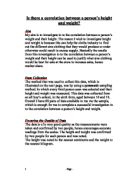
Conclusion
After looking at my results, I have seen that my hypothesis that males are taller than females in average and as you get taller you become heavier has generally been proven to be correct. My diagrams and graphs show clearly that it is correct.
During my collection of information I had to adjust some of my tables and graphs due to anomalous data. My box and whisker diagrams showed and cumulative frequency chart showed clear easy comparison between genders and so were easy to compare results. I also realised once I had plotted the box and whisker diagrams that the data had a big range but almost all of the data was inside the upper and lower quartile ranges. I could have improved my investigation by collecting data of year 7 pupils and perform the same actions I did with my investigation and compare them together.
I also concluded from plan one that simply, as height increases, weight increases. This lead onto separating out the years which concluded that the amount that the pupils grew per school year increased as the year increased. Due to a school year being discreet data, I compared height to weight. However, as weight can continue to increase after a pupil’s teenage years, and from real life experience and my own knowledge, the height cannot be controlled it usually always stops and sometimes reverses. The weight can be controlled by a pupil consuming more or less which can suggest that there cannot be a fully justifiable conclusion made that can relate to everybody in the population as one of the variables can be directly controlled by a human being and the other variable cannot. However, apart from this, I can conclude that the majority of the population prove that my hypothesis is correct: as the height increases, the weight increases – it is directly proportional.
If I was to repeat this investigation, I would choose another year to investigate, as after a few years children have grown to their typical height.