If we are going to draw a histogram to represent the data, we first need to find the class boundaries. In this case they are 5, 11, 16 and 18. The class widths are therefore 6, 5 and 2.
The area of a histogram represents the frequency.
The areas of our bars should therefore be 6, 15 and 4.
This information can be marked on the grid.
A frequency polygon is an easy way of comparing two sets of data frequencies as they can be drawn on the same graph. This means that they are an easy way of finding the modal group as well as the skew (trend of a frequency polygon).
My Hypotheses
A hypothesis is the outline of the idea/ideas which I will be testing and below are the following hypotheses I have decide to investigate for this particular piece of coursework.
- The cleverer you are the higher your maths level
- The needed stratified data
- A scatter diagram
- The correlation coefficient
- Boys are taller and weigh more on average in comparison to girls.
- Cumulative frequency diagram with box plots.
- Average, median, mode and range.
- Frequency polygons (to show the distribution)
- Upper quartile, lower quartile and inter-quartile range
- Mean and standard deviation.
The pre-test
A pre-test or a pilot study is a test of a full scale study. I will use it to check if my first hypothesis will work. I will do it on a much smaller scale and see if it my hypothesis has a positive, negative, or no correlation, If the hypothesis does not have a correlation than I will use a different hypothesis.
First I will use stratified sampling to find the right amount of students. A stratified sample takes a proportional number from each group in the population so that each group is fairly represented. This is necessary when producing graphs or statistical calculations on more than one section of the population together.
No. of each group in sample =
All the following have been rounded.
Year 7 boys = 151/1183 x 25 = 3
Year 7 girls = 131/1183 x 25 = 3
Year 8 boys = 145/1183 x 25 = 3
Year 8 girls = 125/1183 x 25 = 2
Year 9 boys = 118/1183 x 25 = 2
Year 9 girls = 143/1183 x 25 = 3
Year 10 boys = 106/1183 x 25 = 2
Year 10 girls = 94/1183 x 25 = 2
Year 11 boys = 84/1183 x 25 = 2
Year 11 girls = 86 / 1183 x 25 = 2
Now I know how much of each year group and gender I will use. However to eliminate bias I must pick randomly. I can do this by entering the following into a scientific calculator.
Ran# X how Much students there are in my group.
E.g. Ran x (131 females in year 10) = this will give me random number between 1 and 131.
I have found the random stratified numbers from each group as my first hypothesis requires IQ and maths level. I have deleted the rest of the data.
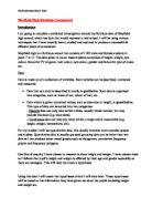
Now I will draw a scatter gram and line of best fit to find the correlation of my hypothesis.
This scatter graph shows that there is a positive correlation between IQ and Maths level. I will continue with my line of enquiry.
Main study- hypothesis 1 - The cleverer you are the higher your maths level
For my main study I have sampled on a much larger scale. I have dealt with all the 10 groups separately, in order to make comparisons against year group and gender. I have randomized by using excel.
I am now going to sample using stratified sampling all the random unbiased students from each year group.
Year 7 males 151/1183 x 100 = 13 (R)
Year 7 females 131/1183 x 100 = 11 (R)
Year 8 males 145/1183 x 100 = 12 (R)
Year 8 females 125/1183 x 100 = 11 (R)
Year 9 males 118/1183 x 100 = 10 (R)
Year 9 females 143/1183 x 100 = 12 (R)
Year 10 males 106/1183 x 100 = 9 (R)
Year 10 females 4/1183 x 100 = 8 (R)
Year 11 males 84/1183 x 100 = 7 (R)
Year 11 females 86/1183 x 100 = 7 (R)
Hypothesis 2 - Boys are taller and weigh more on average in comparison to girls
Planning
I have already randomized and eliminated bias from my results using randomisation methods. Therefore I will keep the same pupils that I had chosen in my last hypothesis.
However I will still be using stratified sampling as I need a fair representation of boys and girls. Here is a table I have produced which contains the number of boys and girls in each year.
The table below is a two way table due to the fact that there are two variables shown at the same and helps view results and data conclusively.
I will use stratified sampling to investigate my second hypothesis. This is because it takes into thought all our needs of the sampling of the data; and this method is accessible and can be easily manipulated.
The variable for the sample is gender so I will do separate samples for boys and girls and vary the amount of samples from each year group to keep the sample unbiased. This is done as different year groups had different amount of pupils so it would be unfair to take the same number of samples from each year group i.e. 5 samples out of 55 is not a fair representation of 5 samples out of 200 so stratified sampling will be helpful as it will eliminate this factor.
I will be calculating my stratified sampling by using the table below:
Frequency charts
Now I have my data I will put them into frequency tables to make them easier to read and it is a useful way of representing data and helps view trends within my sampling that I have produced. I will group some of my frequencies as this will help me later when I will create histograms from my data.
About 90% of the boys in my sample have a height of 1.5 to 1.8 metres this shows me that I have a neutral skew of my data.
This tally frequency table shows that like the heights the boys weight has a near perfect neutral skew, it has very high frequencies in the middle groups and very low frequencies in the starting and ending groups. This notifies me that the students in my sample have an average weight as well as average height.
This table shows me that nearly 75% of the female students are between 1.50 to 1.70 metres. It also shows me that the students are slightly tall for their age as there is a positive skew to the frequency. This could be because of the sample I have taken or it could be for the whole school.
Mean and standard deviation of data
I will now find the mean of the frequency that I have found and this will be quick, efficient and reliable and will help me gain evidence on weather boys are taller and weigh more in comparison to girls. I will also include standard deviation of my data. Standard deviation measures the spread of a distribution around the mean. A normal distribution is usually defined by the mean and standard deviation. These parameters give an easy way to summarise data as the sample gets large: 685 of the values are within one standard deviation of the mean. 95% of the values are within two standard deviations of the mean. 99% of the values are within three standard deviations of the mean.
When comparing distributions, it is better to use a measure of spread or dispersion (such as standard deviation) in addition to measure of central tendency (such as mean, median or mode).
For example, the following two data sets are significantly different in nature and yet have the same mean, median and rage. Some sort of numerical measure which distinguishes between them would be useful.
- 1, 7, 12, 15, 20, 22, 28
- 1, 15, 15, 15, 15, 16, 28
Histograms and Frequency polygons - Height
From the data that I have collected and formed through my frequency tables and mean averages etc I will now produce a frequency polygon and histogram that shows the Boys & girls height from my sample that I have taken for my coursework. The frequency polygon will help me clearly identify the spread or the skew of the data and both these forms of data will help me form a sufficient analysis.
Boy’s height
Histogram on graph paper
The following histogram and frequency polygon clearly shows me that the most common height is between 1.50≤h<1.60 m. However I will not rely on this to support my hypothesis as the data is not evenly distributed. I will use other measures as well such as Inter-quartile range as well.
Girl’s height
Now as I have the boy’s histogram and freq polygon and the girl’s histogram and freq polygon I will compare the two hypotheses to see if they support my hypothesis.
Histogram on graph paper
These graphs clearly show that the most common height is 1.60≤h<1.70 m this shows that my hypothesis is not supported by these two graphs. However I will continue by working out the inter-quartile range.
Cumulative frequency diagrams and tables - height
I will now produce a cumulative frequency diagram for both girls and boys heights as this will help me gain vital evidence towards forming my conclusion of the hypothesis.
From this particular diagram I was able to tell that the median is 1.67 m which I believe is average. I will be finding the inter-quartile range which will help me eliminate any anomalies and margin for error
Girl’s height
From this diagram I can tell that the median is 1.64m which supports my hypothesis however I will still be finding the inter-quartile range as this will deal with any anomalous data.
Boys and girls height Box-plots
From the data that I have found by comparing the box plots I found out that the inter-quartile range for the boys is exactly 0.07m higher than that of the girls. I have also found out that the mean for the boys is exactly 0.11m higher than the girls and the median for the boys 0.1m higher than the girls. This shows me that without anomalous results the boys in my sample are on average taller than the girls in my sample. Part of my hypothesis is supported by the evidence.
Boys and girls weight
I will now produce a histogram as well as a frequency polygon for the boys and girls weight, these representations of data will help me find the most common modal class and see if it supports my hypothesis or not.
Boy’s weight
Histogram on graph paper
From this histogram and frequency table I can tell that the modal class of the boys weight is 40≤w<50 Kg.
Girl’s Weight
Histogram on graph paper
The histogram shows me that the most common weight is between 40 – 50 kg. This is the same as the boys and does not support my hypothesis however I will continue by drawing a cumulative frequency diagram and working out the inter-quartile range to see if my hypothesis is correct.
Cumulative frequency diagrams and tables - weight
From this cumulative frequency diagram I can tell that the median of the boy’s weight is 54 kg which is in my opinion slightly less than average.
Girl’s weight
From this graph I can tell that the median for the girls weight is 51 kg this supports my hypothesis that boys are taller than girls however I will continue with more means of analysis such as Box – plots and inter-quartile range to eliminate any anomalous results.
Boys and girls Weight Box-plots
From the data that I have found by comparing the box plots I found out that the inter-quartile range for the boys is exactly 0.75kg higher than that of the girls. I have also found out that the mean for the boys is exactly 2.34kg higher than the girls and the median for the boys 1.5kg higher than the girls. This shows me that without anomalous results the boys in my sample are on average heavier than the girls in my sample.
Conclusion – Hypothesis one
My first hypothesis was “the higher your IQ level the higher your maths level” in this hypothesis I decided to investigate how clever you are with your maths level predicting that a cleverer person will have a higher maths level.
As the entire school was too large for me to analyse I used stratified sampling to sample an equal representation of each gender in each year group. In my pre test I used fairly small samples such as 2-3 for each year group. To eliminate bias I used a calculator function call ran#, this generated random numbers from the school database that I could use. Using the samples I created a scatter graph and a correlation coefficient. The scatter graph showed me that there was a positive correlation for the two variables and the correlation coefficient showed me that there was a good strong correlation of the two, so I continued with my line of enquiry.
In my genuine hypothesis I used stratified sampling on a much larger proportion of the school to create a more reliable result. To eliminate bias I could not use the calculator as it was not efficient and wasted time. So using excel I sorted each year group and gender randomly by using a random sort technique that generates a unique random number for each pupil. Then I using the newly stratified and randomized pupils I created a scatter graph and correlation coefficient. I saw that there was a good positive correlation on my scatter graph and there was a strong positive correlation coefficient. This proved to me that my hypothesis was proved by my results. However nothing in statistics is ever proved, it is just supported by my results.
Evaluation – Hypothesis one
I think that in my first hypothesis my results were accurate, efficient and reliable. I believe that I completed this hypothesis with the best of my ability and I believe that these results could be used to make predictions for all of Mayfield high school as well as schools in general.
In my first hypothesis I did have some limitation as I believe that I should have sampled more people to get better more reliable results. Because if I had more pupils to analyse on then I could have a better representation of the school so it would be more consistent and trustworthy.
While undertaking my first hypothesis I encountered a few problems. The first problem I had was when I was sampling and sorting my data it was very difficult to sort it into a fair order so that I can sample and randomize my pupils. If I was to make any corrections to my hypothesis I would sort it into a fair order to further eliminate bias from my results. The second problem I faced was transferring my sampled pupils in an order so that I can analyse them. This was very difficult as I had to adjust all the data I needed for the pupils so I can create a scatter graph and a correlation coefficient. If I was to do this coursework again I would put my needed data into a sorted order so it would be easier for me to analyse.
Hypothesis 2
As I had already sampled and randomised the pupils I wanted to analyse from the Mayfield high database I used the same pupils I used in hypothesis on as I did in hypothesis 1.
My hypothesis was “boys are taller and weigh more in comparison to girls”, at the start of my hypothesis I created a two way table that showed the year group gender and total gender and year group. Using this I sampled all the boys and girls I needed from my already randomized data. By creating frequency charts I was able to tell the most common class interval of each of the four variables (boy’s height, boy’s weight, girl’s height, and girl’s weight).
Afterwards using frequency tables I found the mean and standard deviation of each of the four variables I found that the standard deviation for the girls was exactly 2.08 higher than of the boys this showed me that the girl’s weight was more spread out about the mean than the boys. I also found that the standard deviation for the girls height was exactly 0.061 higher than the boys. This again showed me that the girl’s height is more spread about the mean.
Subsequently I used a software program to create visual representations of the variables such as histograms and frequency polygons, both graphs helped me in identifying trends within the data. I also drew cumulative frequency diagrams as this helped me to identify the inter-quartile range as well as the quartiles.
After that I used box plots mad by using the cumulative frequency diagrams to compare boy’s height with girl’s height and boy’s weight to girl’s weight. This was an excellent way to compare them because it compared the median, mode and the inter-quartile range visually.
From the results I can conclude that:
My results support that boys are heavier than girls as the inter-quartile range for the boys is exactly 0.75kg higher than that of the girls (making sure there are no anomalous results), that the mean for the boys is exactly 2.34kg higher than the girls and the median for the boys 1.5kg higher than the girls. My evidence supports that boys are taller than girls as the inter-quartile range for the boys is exactly 0.07m higher than that of the girls, the mean for the boys is exactly 0.11m higher than the girls and the median for the boys 0.1m higher than the girls. Girl’s height and weight has more spread about the mean than of the boy’s height and weight.
Evaluation
I believe that the results I analyzed from my sample are not a fair representation of my sample because I believe that as there were too many factors involved in randomizing, sorting and creating graphs etc that my results may have been incorrect or biased in some way or the other.
In my hypothesis I believe that there were a few limitations that if I believe I exceeded I would have more efficient, accurate and reliable results. Such as if I sampled more than 100 students my results would have been more reliable. I also believe that if I analysed my data more I would have more accurate results using methods such as correlation coefficient and spearman rank correlation.
When I was undertaking this hypothesis I faced a few problems which I believe could have been avoided. Firstly I believe that I could have organized my data better so it could have been analysed easily giving me better unbiased results. Such as putting my sampled data into order such as year group, gender, height and weight this would have been more efficient and would have saved a lot of time. Secondly I believe that I did not use my time effectively with this hypothesis because the articles I needed to spend less time on I spent more time on them and the articles I should’ve spent more time on I spent less time on. If I was to do this hypothesis again I would use my time more efficiently.