Secondly, we must establish an equation for the time taken for the ball to come to rest.
If we use the following model for the time taken for the ball to bounce, an equation can be established.
For the first bounce, the following can be said:
u = ev a = -g
v = -ev t = ?
Using the equation of linear motion v = u + at
-ev = ev – gt
t =
For the second bounce, the following can be said:
u = e2v a = -g v = -e2v t = ?
Again, using v = u + at:
-e2v = e2v – gt
t =
From this, it can be seen that a geometric progression is occuring in the form:
t = t0 + + + …
The forumula for the sum to infinity of a geometic progression can be used.
∑ =
In this case, r = e and a = t0. As e will never take values greater than 1, it satisfies the requirement that |r| = 1 for the above formula. This then gives the following formula:
∑ =
To complete this model, we need to define t0 in terms of h0 (the initial drop height). This needs to be in terms of the height that the ball is dropped from (as opposed to the time in seconds the first drop takes).
When dropping the ball:
a = g u = 0 v = 2h0g t = ?
Using v = u + at
2hog = 0 + gt
t =
From this, the final equation for the sum time can be established:
∑ =
Where h is the initial drop height, g is the gravitational pull (at 9.8ms-1 and e is the elasticity (which is found using the first equation obtained in terms of h1 and h2)
Conducting the Experiment
Method:
Other methods used to reduce the experimenter errors were to have two people checking the rebound height – this lowers the chance of experimenter judgement affecting the results adversely. The whole method process was used for both the rebound heights and time taken to stop bouncing. The results are shown on the following page.
Results:
Experiment One – rebound height (in cms)
Experiment Two – Time Taken to stop bouncing (in seconds)
Applying the model to the results
For values of e:
Using the first equation,
e =
Using the graph, values for the maximum, minimum and mean gradients can be obtained, thus giving maximum, minimum and mean values of e.
Mean value of e =
e = 0.75 to 2 d.p
Maximum value of e =
e = 0.77 to 2 d.p
Minimum value of e =
e = 0.72 to 2 d.p
Using the values of e, we can now obtain the time taken for the ball to stop bouncing, using the second modelled equation, if we take the value of e to be the mean (of 0.75) and the height to be 100cm:
∑ =
∑ = 8 seconds
The same technique can be used for the other results, which are displayed in the following table:
Mean Actual Times and Mean e:
We can adjust the time model to take the values for the maximum and minimum of e:
Maximum Actual Times and Maximum e:
Minimum Actual Times and Minimum e:
Discussion of Variation in Results
From the quantitative data obtained from the experiments, and observing the graphs, it can be seen that the results for the 100cm condition when measuring the bounce may have been somewhat flawed. This, in turn, will have increased the values of e for the maximum and mean. However, the minimum would be unaffected, as the maximum value for 100cm was not used for this gradient measure.
Also, it can be noted that there is a fairly significant variation in the results for the rebound heights. For example, with the 20cm drop height; the difference between results is 5cm. This is not such a problem with the times, as they appear to be within a few tenths of a second within each other.
Comparison between experimental results and predictions of the model
Using the experimental result for the value of e, the modelled times taken for the ball to stop bouncing are different from that of the actual results. This is shown in the table below:
Mean Values:
Maximum Values:
Minimum Values:
Graphical Representations:
Mean:
Maximum:
Minimum:
It can be said that the model times are approximately half that of the actual (mean) times. However, as the drop height becomes smaller, the model and actual times appear to converge slightly.
The primary reason for the model giving smaller times than the mean, maximum and minimum times is because the model assumes that the mass is a particle (one of the assumptions outlined at the start of this investigation). It does not account for mass or air resistance, which may both affect the model, thus causing the model to perhaps give results similar to the actual results.
Experimenter effects are another reason for the differences between the model and the actual times. By simply observing the graphs, effects which cause such a gap in the times may include the experimenter’s definition of when the ball actually “stops” bouncing, the true height from which the ball was dropped from and the slight difference that may occur between the ball dropping and the stopwatch being started, even though this was done by the same experimenter.
Initial results indicated that taking the means, and rounding them to 2.d.p may have caused the difference between the model and the actual results. However, workings have taken place using the maximum and minimum times and values of e, which also show a similar difference between the model and the actual results.
Revision of the process
In order to improve the model:
- Fewer assumptions would be used
- Air resistance would be taken into account
- Also the fact that the ball is not a fixed particle needs to be taken into account – this is a major contributing factor to the difference between the model and the results.
In order to improve the experiment:
- Take more measurements for the times and rebound heights.
- Use a technological method to measure the times and rebound heights to increase the validity of the results.
- Increase the accuracy of the value of gravity.
The effects that these amendments would have are that the accuracy of the results would be increased. This, in turn, would mean the value of e would be more exact, thus giving a model that gives times closer to the experimental times.