P(X=0) = 5 (0.5733)0 (0.4267)5 = 0.0141
0
P(X=1) = 5 (0.5733)¹ (0.4267)4 = 0.0951
1
P(X=2) = 5 (0.5733)² (0.4627)³ = 0.2553
2
P(X=3) = 5 (0.5733)³ (0.4627)² = 0.3431
3
P(X=4) =5 (0.5733)4 (0.4627)1= 0.2305
4
P(X=5) = 5 (0.5733)5 (0.4627)0 = 0.0619
5
Therefore the expected frequencies are: 0.0141 x 15 = 0.212
0.0951 x 15 = 1.42
0.2553 x 15 = 3.83
0.3431 x 15 = 5.15
0.2305 x 15 = 3.46
0.0619 x 15 = 0.929
Family Of Six
Number of families = 9
Total number of children = 54
Number of boys = 24
Probability of male birth = 24/54 = 0.4444
Therefore probability of female birth = 1-0.4444 = 0.55555
P(X=0) = 6 (0.4444)0 (0.5555)6 = 0.0294
0
P(X=1) = 6 (0.4444)¹ (0.5555)5 = 0.1411
1
P(X=2) = 6 (0.4444)² (0.5555)4 = 0.2822
2
P(X=3) = 6 (0.4444)³ (0.5555)³ = 0.3009
3
P(X=4) = 6 (0.4444)4 (0.5555)² = 0.1796
4
P(X=5) = 6 (0.4444)5 (0.5555)¹ = 0.0578
5
P(X=6) = 6 (0.4444)6 (0.5555)0 = 0.0077
6
Therefore the expected frequencies are: 0.0294 x 9 = 0.26
0.1411 x 9 = 1.27
0.2822 x 9 = 2.54
0.3009 x 9 = 2.71
0.1796 x 9 = 1.62
0.0578 x 9 = 0.52
0.0077 x 9 = 0.069
On the whole the above data suggests that generally there is a greater probability of a female birth than a male birth.
The tables below show the comparison between the expected frequencies and the observed frequencies.
Family Of One
Family Of Two
Family Of Three
Family Of Four
Family Of Five
Family Of Six
Chi-Squared Test
Family Of One
(25-25)² + (24-24)² = 0
- 24
In this investigation there are two constraints, the total number of families and the probability There are two cells and two constraints, therefore there are no degrees of freedom, the model fits the data perfectly as the value of the chi-squared test is 0.
Family Of Two
(32-33.77)² + (74-70.468)² + (35-36.77)²
33.77 70.468 36.77
= 0.092772 + 0.177031 + 0.0852026
=0.355
Again there are two constraints, but this time three cells so there is one degree of freedom. By using the X² table of values, at the 10% level it gives a value of 2.71, my value is 0.355 this indicates that the model fits the data extremely well as well over 10% of the values will be less than 2.71.
Family Of Three
(23-20.29)² + (56-57.71)² + (50-54.71)² + (21.17.29)²
20.29 57.71 54.71 17.29
= 0.361957 + 0.0506689 + 0.405853 + 0.796073
= 1.61
There are 2 constraints and four cells, this means there are two degrees of freedom, in the table the value for 10% is 4.61, compared to my value of 1.61this indicates that the model, once again, fits the data extremely well.
Family Of Four
(8-8.5)² + (29-26.7)² + (32-31.296)² + (10-16.32)² + (7-3)²
8.5 26.7 31.296 16.32 3
=8.026
Again there are two constraints five cells, this gives three degrees of freedom, at the 10% level in the table the value is 6.25 compared to my value of 8.026this suggests that the model fits the data quite well but it is not as good a fit as in the previous family sizes.
Family Of Five
(0-0.212)² + (1-1.42)² + (5-3.53)² + (4-5.15)² + (5-3.46)² + (0-0.929)²
0.212 1.42 3.53 5.15 3.46 0.929
=2.56
With two constraints and 6 cells there are 4 degrees of freedom. At the 10% level the value in the table is 7.78. This therefore proves that the model fits the data very well as my value was just 2.56. This means that well over 10% of the values will be below 7.78 so there will be a high percentage of values around 2.56.
Family Of Six
(0-0.26)² + (2-1.27)² + (1-2.54)² + (5-2.7)² + (0-1.62)² + (1-0.52)² + (0-0.069)²
0.26 1.27 2.54 2.7 1.62 0.52 0.069
= 5.26
There are two constraints and seven cells. This gives 5 degrees of freedom. In the table the 10% value is 9.24 comparing it with my value of 5.26 suggests that the model once again fits the data very well.
All in all from this part of my investigation I feel that I can say the binomial model fits my data very well.
To investigate family size further I am going to alter my working out by using the probability found in the unit text book.
Using Equal Probability Of Male/Female Birth.
By using the binomial model I can work out the expected probability/frequency of X number of male births in each family size.
Family Of One
Number of families = 49
Probability of male birth = 0.5
Probability of female birth = 0.5
P(X=0) = 1 (0.5)0 (0.5)¹ =0.5
0
P(X=1) = 1 (0.5)¹ (0.5)0 =0.5
1
Therefore the expected frequencies are: 0.5 x 49 = 24.5
0.5 x 49 = 24.5
Family Of Two
Number of families = 141
Probability of male birth = 0.5
Probability of female birth = 0.5
P(X=0) = 2 (0.5)0 (0.5)² = 0.25
0
P(X=1) = 2 (0.5)¹ (0.5)¹ = 0.5
1
P(X=2) = 2 (0.5)² (0.5)0 = 0.25
2
Therefore the expected frequencies are: 0.25 x 141 = 35.25
0.5 x 141 = 71
0.25 x 141 = 35.25
Family Of Three
Number of families = 150
Probability of male birth = 0.5
Probability of female birth = 0.5
P(X=0) = 3 (0.5)0 (0.5)³ = 0.125
0
P(X=1) = 3 (0.5)¹ (0.5)² = 0.375
1
P(X=2) = 3 (0.5)² (0.5)¹ = 0.375
2
P(X=3) = 3 (0.5)³ (0.5)0 = 0.125
3
Therefore the expected frequencies are: 0.125 x 150 = 18.75
0.375 x 150 = 56.25
0.375 x 150 = 56.25
0.125 x 150 = 18.75
Family Of Four
Number of families = 86
Probability of male birth = 0.5
Probability of female birth = 0.5
P(X=0) = 4 (0.5)0 (0.5)4 = 0.0625
0
P(X=1) = 4 (0.5)¹ (0.5)³ = 0.25
1
P(X=2) = 4 (0.5)² (0.5)² = 0.375
2
P(X=3) = 4 (0.5)³ (0.5)¹ = 0.25
3
P(X=4) = 4 (0.5)4 (0.5)0 0.0625
Therefore the expected probabilities are: 0.0625 x 86 = 5.375
0.25 x 86 = 21.5
0.375 x 86 = 32.25
0.25 x 86 = 21.5
0.0625 x 86 =5.375
Family Of Five
Number of families = 15
Probability of male birth = 0.5
Probability of female birth = 0.5
P(X=0) = 5 (0.5)0 (0.5)5 = 0.03125
0
P(X=1) = 5 (0.5)¹ (0.5)4 = 0.15625
1
P(X=2) = 5 (0.5)² (0.5)³ = 0.3125
2
P(X=3) = 5 (0.5)³ (0.5)² = 0.3125
3
P(X=4) = 5 (0.5)4 (0.5)¹ = 0.15625
4
P(X=5) = 5 (0.5)5 (0.5)0 = 0.03125
The expected frequencies are therefore: 0.03125 x 15 = 0.46875
0.15625 x 15 = 2.3
0.3125 x 15 = 4.6875
0.3125 x 15 = 4.6875
0.15625 x 15 = 2.3
0.03125 x 15 = 0.46875
Family Of Six
Number of families = 9
Probability of male birth = 0.5
Probability of female birth = 0.5
P(X=0) = 6 (0.5)0 (0.5)6 = 0.015625
0
P(X=1) = 6 (0.5)¹ (0.5)5 = 0.09375
1
P(X=2) = 6 (0.5)² (0.5)4 = 0.234
2
P(X=3) = 6 (0.5)³ (0.5)³ = 0.3125
3
P(X=4) = 6 (0.5)4 (0.5)² = 0.234
4
P(X=5) = 6 (0.5)5 (0.5)¹ = 0.09375
5
P(X=6) = 6 (0.5)6 (0.5)0 = 0.015625
6
Expected frequencies are: 0.015625 x 9= 0.1466
0.09375 x 9 = 0.8438
0.234 x 9 = 2.106
0.3125 x 9 = 2.8125
0.234 x 9 = 2.106
0.09375 x 9 = 0.8438
0.015625 x 9 = 0.1466
The tables below show the comparison between the observed frequencies and the expected frequencies.
Family Of One
Family Of Two
Family Of Three
Family Of Four
Family Of Five
Family Of Six
Chi-Squared Test.
Family Of One.
(25-24.5)² + (24-24.5)²
- 24.5
=0.02041
There is one constraint in this investigation, the total number of families. There are two cells and therefore 1 degree of freedom. At the 10% level the value in the table is 2.71, compared with my figure above the model fits the data extremely well.
Family Of Two
(32-35.25)² + (74-70.5)² + (35-35.25)²
35.25 70.5 35.25
= 0.3839
There are three cells and one constraint giving two degrees of freedom, the 10% value is 4.61. This shows that the model fits the data almost perfectly.
Family Of Three
(23-18.75)² + (56-56.25)² + (50-56.25)² + (21-18.75)²
18.75 56.25 56.25 18.75
= 1.695
There are three degrees of freedom because the are four cells and one constraint. The table gives a value of 6.25 at the 10% level, this suggests the model fits the data well.
Family Of Four
(8-5.375)² + (29-21.5)² + (32-32.25)² + (10-21.5)² + (7-5.375)²
5.375 21.5 32.25 21.5 5.375
= 11.37
In this instance there are four degrees of freedom. At the 2.5% level the value in the table is 11.4 this suggests that the model does not fit the data particularly well.
Family Of Five
(0-0.46875)² + (1-2.3)² + (5-4.6875)² + (4-4.6875)² + (5-2.3)² + (0-0.46875)
0.46875 2.3 4.6875 4.6875 2.3 0.46875
= 4.1198
There are five degrees of freedom and seeing as the 10% value in the table is 9.24 this suggests that the model, again, fits the data very well.
Family Of Six
(0-0.147)² + (2-0.844)² + (1-2.11)² + (5-2.813)² + (0-2.11)² + (1-0.844)² + (0-0.147)²
0.147 0.844 2.11 2.813 2.11 0.844 0.147
= 4.8333
There are six degrees of freedom due to the one constraint and the seven cells. The value given in the table at the 10% level is 10.64, compared to my figure it above this shows that the model is a very good fit for the data.
The final modification I can make to my model is altering the probabilities to the others stated in the textbook.
Using Probabilities From The Census.
Family Of One
Number of families = 49
Probability of male birth = 0.513
Probability of female birth = 0.487
P(X=0) = 1 (0.513)0 (0.487)1 = 0.487
0
P(X=1) = 1 (0.513)1 (0.487)0 = 0.513
1
Expected frequencies are: 0.487 x 49 = 23.863
0.513 x 49 = 25.137
Family Of Two
Number of families = 141
Probability of male birth = 0.513
Probability of female birth = 0.487
P(X=0) = 2 (0.513)0 (0.487)² = 0.237
0
P(X=1) = 2 (0.513)¹ (0.487)¹ = 0.4997
1
P(X=2) = 2 (0.513)² (0.487)0 = 0.263
Expected frequencies are: 0.237 x 141 = 33.44
0.4997 x 141 = 70.45
0.263 x 141 = 37.1
Family Of Three
Number of families = 150
Probability of male birth = 0.513
Probability of female birth = 0.487
P(X=0) = 3 (0.513)0 (0.487)³ = 0.116
0
P(X=1) = 3 (0.513)¹ (0.487)² = 0.365
1
P(X=2) = 3 (0.513)² (0.487)¹ = 0.384
2
P(X=3) = 3 (0.513)³ (0.487)0 = 0.1350
3
Expected frequencies are: 0.116 x 150 = 17.325
0.365 x 150 = 54.75
0.384 x 150 = 57.67
0.135 x 150 = 20.25
Family Of Four
Number of families = 86
Probability of male birth = 0.513
Probability of female birth = 0.487
P(X=0) = 4 (0.513)0 (0.487)4 = 0.0562
0
P(X=1) = 4 (0513)¹ (0.487)³ = 0.237
1
P(X=2) = 4 (0.513)² (0.487)² = 0.374
2
P(X=3) = 4 (0.513)³ (0.487)¹ = 0.263
3
P(X=4) = 4 (0.513)4 (0.487)0 = 0.0693
Expected frequencies are: 0.0562 x 86 = 4.84
0.237 x 86 = 20.38
0.374 x 86 = 32.21
0.263 x 86 = 22.62
0.0693 x 86 = 5.9
Family Of Five
Number of families = 15
Probability of male birth = 0.513
Probability of female birth = 0.487
P(X=0) = 5 (0.513)0 (0.487)5 = 0.0274
0
P(X=1) = 5 (0.513)¹ (0.487)4 = 0.144
1
P(X=2) = 5 (0.513)² (0.487)³ = 0.304
2
P(X=3) = 5 (0.513)³ (0.487)² = 0.321
3
P(X=4) = 5 (0.513)4 (0.487)¹ = 0.169
4
P(X=5) = 5 (0.513)5 (0.487)0 = 0.0355
5
Expected frequencies are: 0.0274 x 15 = 0.411
0.144 x 15 = 2.16
0.304 x 15 = 4.56
0.321 x 15 = 4.80
0.169 x 15 = 2.53
0.0355 x 15 = 0.53
Family Of Six
Number of families = 9
Probability of male birth = 0.513
Probability of female birth = 0.487
P(X=0) = 6 (0.513)0 (0.487)6 = 0.0133
0
P(X=1) = 6 (0.513)¹ (0.487)5 = 0.0843
1
P(X=2) = 6 (0.513)² (0.487)4 = 0.222
2
P(X=3) = 6 (0.513)³ (0.487)³ = 0.312
3
P(X=4) = 6 (0.513)4 (0.487)² = 0.246
4
P(X=5) = 6 (0.513)5 (0.487)¹ = 0.104
5
P(X=6) = 6 (0.513)6 (0.487)0 = 0.0182
6
Expected frequencies are: 0.0133 x 9 = 0.12
0.0843 x 9 = 0.76
0.222 x 9 =1.998
0.312 x 9 = 2.81
0.246 x 9 = 2.22
0.110 x 9 = 0.93
0.0182 x 9 = 0.16
The tables below show the comparison between the observed frequencies and the expected frequencies.
Family Of One
Family Of Two
This shows that in a family of two you would expect to find that around half of the families had one boy in them.
Family Of Three
This shows that for a family of three you would expect the majority of families to have either one or two boys. According to my data you would expect more to have one boy, but according to the expected frequencies it would be the other way round.
Family Of Four
My data suggests that the majority of families will have 2 boys in them
Family Of Five
This shows that you would expect to find more families with 2,3 or 4 boys in them.
Family Of Six
This suggests that the majority of families will have three boys in them.
The Chi-Squared Test
Family Of One
(25-23.863)² + (24-25.137)²
- 25.137
= 0.1056
There are two cells and one constraint giving one degree of freedom. In the table the value representing 10% is 2.71, this indicates that the model fits the data very well.
Family Of Two
(32-33.44)² + (74-70.45)² + (35-37.1)²
33.44 70.45 37.1
= 0.3598
There are two degrees of freedom due to there being three cells and the one constraint (number of families). The 10% value in the table of 4.61 shows that the binomial model fits the data extremely well.
Family Of Three
(23-17.325)² + (56-54.75)² + (50-57.67)² + (20-20.251)²
17.352 54.75 57.67 20.251
= 3.989
There is once again one constraint and this time four cells. This gives three degrees of freedom. The value representing 10% is 6.25. This indicates that the model is a good fit for the data as well over 10% of the figures will be below 6.25
Family Of Four
(8-4.84)² + (29-20.38)² + (32-32.21)² + (10-22.62)² + (7-5.9)²
4.84 20.38 32.21 22.62 5.9
= 13.36
The figure at the 2.5% level is 12.83, this suggests that the model is not that good a fit for the data as only a small proportion of the data will be around 13.36
Family Of Five
(0-0.411)² + (1-2.16)² + (5-4.56)² + (4-4.80)² + (5-2.53)² + (0-0.53)²
0.411 2.16 4.56 4.80 2.53 0.53
= 1.5333
There are five degrees of freedom which gives a 10% value of 9.24 suggesting that the model fits the data extremely well.
Family Of Six
(0-0.12)² + (2-0.76)² + (1-1.998)² + (5-2.81)² + (0-2.22)² + (1-0.93)² + (0-0.16)²
0.12 0.76 1.998 2.81 2.22 0.93 0.16
= 4.833
There are six degrees of freedom. The table gives a 10% value of 10.64 suggesting that the binomial model is a very good fit for the data as well over 10% of the values will be less than 10.64.
If you compare the chi-squared tests for each of the three different probabilities it is clear to see that the one using the probabilities calculated from the data fits the model the best. This will be because it is more true to life and is worked out using the data itself, not statistics found in a book.
Below is a table comparing the chi-squared tests.
As you can see the Chi-squared test fits the model better when using the probabilities calculated from the data for families of one, two, three and four. I would suggest that it does not fit the data as well for families of five and six because I only had a very small sample of data for these family sizes. The binomial model fits the data better for families of one and two than any other family size.
Generally you can say that the binomial model fitted the probability model very well no matter what probabilities were used.
I also decided to calculate the mean number of boys in each family size, to do this I totalled up the number of boys in the family size and divided it by the number of families. The results were as follows:
Family Of One:- mean = 24/49 = 0.4897
Family Of Two:- mean = 144/141 = 1.02
Family Of Three:- mean = 219/150 = 1.46
Family Of Four:- mean = 151/86 = 1.76
Family Of Five:- mean = 43/15 = 2.86667
Family Of Six:- mean = 24/9 = 2.6667.
As you would expect, this shows an increase in the average number of boys up until families of six, this is probably because I only had a small amount of data for this family size, hence an anomalous result was found.
I Could then also analyse the family sizes themselves. To do this a constructed a contingency table. To work out the expected frequencies of each family size I multiplied the number of
families in each size group, by the number of children in that size group. I then divided this figure by the total number of children, which in my investigation was 1254 and then multiplied that answer by the total number of families which is 450. The results are shown below.
I then did the chi-squared test on this data following the same method as before. This gave me a value of 89.12. In this investigation there is one constraint, the total number of families, this gives 5 degrees of freedom. In the table of values the 0.1% value for 5 degrees of freedom is 20.52. This suggests that the model is not a good fit for the data when it is considered as one big set of data and not split up into different family sizes. This is probably because for some family sizes only a small amount of data was collected. However I feel that I can say from the data I collected that the most commonly found family sizes are families of 2, 3 and 4.
If I were to do this investigation again I would take a larger sample of families and perhaps make sure that I had sufficient data to analyse it. The fact that I only had 15 families of 5 and nine families of 6 meant that it was very hard for me to analyse this data, it may have been better if I had decided either to group families of five and six together or not included them in the investigation due to insufficient numbers. The probabilities taken from the census may no longer be true to life because the census was taken 10 years ago and the statistic may have changed, this may make the data inaccurate although I do believe it will not make too much of a difference because the difference between the 0.5 probability and 0.513 probability is only small. I would also try to find another way of analysing family sizes on a whole as I feel that my method above is not that conclusive. All in all I feel that my investigation shows that, on the whole, the binomial model does fit the data I collected and it allowed me to make conclusive comments on the structure of families.
DATA