Delete the unwanted cells, for example eye colour and favourite colour.
Results and observations
A stratified sample of 30% of both females and males weights.
This stratified sample also enabled me to get a more varied results from years 7-11.
Based on the number given of males and females in my stratified sample I am going to use these samples of 30% of each gender in order to make my frequency density histogram of the males and females weights
During this I used a fixed random number using a excel worksheet to work out and show that the sample I was going to be using was as accurate as possible to get a more reliable results and prove that my hypothesis is correct.
Errors:
These are the pupils who have errors in there weight because it is very unlikely that someone would have the weight of 5kg, 6kg or 9kg.
The pupil ‘Masooma Abbas’ also is a error in weight because they have no weight.
Anomalies:
This is the pupils who has an anomalies due to her weight because it is unlikely that a year 7 pupil will weigh 140kg
Results and observations:
Stem and Leaf Diagram showing the weights of 173 females:
10:
20:
30: 3 4 5 5 5 5 6 6 8 8 8 8 9
40: 0 0 0 0 0 0 0 0 0 0 1 1 1 2 2 2 2 2 2 2 2 2 3 3 4 4 5 5 5 5 5 5 5 5 5 5 5 5 5 5 6 6 6 6 6 7 7 7 7 7 7 7 7 8 8 8 8 8 8 8 8 8 8 8 8 8 8 8 8 8 8 9 9 9 9 9
50: 0 0 0 0 0 0 0 0 0 0 0 0 1 1 1 1 2 2 2 2 2 2 2 2 2 2 3 3 3 4 4 4 4 4 4 4 4 4 4 4 4 5 5 5 5 5 5 5 6 6 6 7 7 7 8 8 8 8 9 9 9
60: 0 0 0 0 1 1 2 2 3 3 4 5 5 5 5 5 6 6 7
70: 0 2 2 4
80:
90:
Stem and leaf diagram showing the weight of 173 females with modified intervals.
20:
30: 3 4 5 5 5 5 6 6 8 8 8 8 9
40: 0 0 0 0 0 0 0 0 0 0 1 1 1 2 2 2 2 2 2 2 2 2 3 3
44: 0 0 1 1 1 1 1 1 1 1 1 1 1 1 1 1 2 2 2 2 2 3 3 3 3 3 3 3 3
48: 0 0 0 0 0 0 0 0 0 0 0 0 0 0 0 0 0 0 1 1 1 1 1 2 2 2 2 2 2 2 2 2 2 2 2 3 3 3 3
52: 0 0 0 0 0 0 0 0 0 0 1 1 1 2 2 2 2 2 2 2 2 2 2 2 2 3 3 3 3 3 3 3 4 4 4 5 5 5 6 6 66 7 7 7
60: 0 0 0 0 0 01 1 1 2 2 3 3 4 5 5 5 5 5
70: 0 2 2 4
80:
In order to get better results I have had to modify the group boundaries on my first stem and leaf diagram so that I could get more accurate results and graph.
When looking at a stem and leaf diagram, you are not able to get a good indication or extra results however you can see the group boundaries used for your histogram and a general idea of how the histogram will be set out.
This histogram shows the weights of approximately 173 girls from years 7-11 taken from Mayfield school.
This histogram shows
A results box for 173 girls.
Raw Data Statistics:
Number in sample, n: 173
Mean, x: 49.9538
Standard Deviation, x: 8.19828
Range, x: 41
Lower Quartile: 45
Median: 49
Upper Quartile: 54.5
Semi I.Q. Range: 4.75
The results contained in this results box suggest that girls have a overall range of 41 meaning that the range is much shorter than the males.
This histogram shows a random sample of 181 Males weights from years 7-11 taken from Mayfield school.
This histogram has been evenly spread out in the middle so that it can relate more to my tree diagrams
The results box for 181 random male samples.
Raw Data Statistics:
Number in sample, n: 181
Mean, x: 52.768
Standard Deviation, x: 11.3814
Range, x: 64
Lower Quartile: 45
Median: 50
Upper Quartile: 60
Semi I.Q. Range: 7.5
The results contained in this results box suggest that the overall range is 64 which is a lot larger of that of the Females. The mean of 52.768 is higher than the Females of 49.9538
An unordered stem and leaf diagram showing the weights of 181 males.
0:
10:
20: 6 9
30: 1 2 5 5 8 8 8 8 8 9 9
40: 0 0 0 0 0 0 0 1 1 1 1 1 1 2 2 2 2 3 3 3 3 3 4 4 4 4 5 5 5 5 5 5 5 5 5 5 5 5 5 5 5 5 6 6 6 7 7 7 7 7 7 7 7 8 8 8 8 8 8 8 8 8 8 8 9 9 9 9 9 9
50: 0 0 0 0 0 0 0 0 0 0 1 1 1 1 1 1 2 2 2 2 2 2 3 4 4 4 4 5 5 5 5 5 6 6 6 6 6 6 6 6 7 7 7 8 9 9 9 9 9 9
60: 0 0 0 0 0 0 0 0 0 1 2 2 2 2 3 3 3 4 4 4 5 5 5 6 6 8 8 8 9 9 9
70: 0 0 0 2 2 2 2 2 3 5 6 7
80: 0 0 6 6
90: 0
A ordered stem and leaf diagram to show a random sample of 181
0:
10:
20: 6 9
30: 1 2 5 5 8 8 8 8 8 9 9
40: 0 0 0 0 0 0 0 1 1 1 1 1 1 2 2 2 2 3 3 3 3 3
44: 0 0 0 0 1 1 1 1 1 1 1 1 1 1 1 1 1 1 1 1 2 2 2 3 3 3 3 3 3 3 3
48: 0 0 0 0 0 0 0 0 0 0 0 1 1 1 1 1 1 2 2 2 2 2 2 2 2 2 2 3 3 3 3 3 3
52: 0 0 0 0 0 0 1 2 2 2 2 3 3 3 3 3
56: 0 0 0 0 0 0 0 0 1 1 1 2 3 3 3 3 3 3
60: 0 0 0 0 0 0 0 0 0 1 2 2 2 2 3 3 3 4 4 4 5 5 5 6 6 8 8 8 9 9 9
70: 0 0 0 2 2 2 2 2 3 5 6 7
80: 0 0 6 6
90: 0
Like the girls stem and leaf, I ordered these results as well, I changed the group boundaries so that I could get more accurate results.
From this stem and leaf diagram I can see how the histogram will be set out, when looking at the shape of the numbers turned on a angle points upwards you can see your eventual histogram.
A frequency polygon comparing the range and frequency of the males and females weight.
Boy’s weight
Girl’s weights
This shows how the boys have a much larger spread of weight compared to the girls. However the girls have a higher frequency of weights.
This also shows that the males and the females have approximately the same average in weight.
A box plot showing the weights of the random samples of 181 males and 173 females.
This box plot shows that the males have a larger range in data compared to the males, although the females have a smaller median.
The medium contained on this graph strongly shows that there is a very small difference between them, the females have a medium of 49 whereas the males have a medium of 50.
There is also a substantial difference between the quartiles; the
Males
Lower Quartile: 45
Upper Quartile: 60
Females
Lower Quartile: 45
Upper Quartile: 54.5
As we can see, the males have a large upper quartile than the females.
Conclusion:
Now that I have studied Hypothesis 1 I can say that I believe this statement, this is evident in my box and whisker diagrams because the medium is larger meaning that the average weight is generally higher. This is also evident in the histogram because you can see that the bars are generally closer together and not as spread out along the x-axis.
I can also say that my Hypothesis 2 is correct as well, this is evident when looking at the histograms because unlike the Females, the data is generally situated in the centre of the graph whereas the males is more widely spread out.
Evaluation:
If I was going to repeat this investigation again I would change