Statistics Is there a correlation between 100m times and shot-put distances compared to BMI (Body Mass Index)?
GCSE Statistics Coursework
Introduction
Project Title: Is there a correlation between 100m times and shot-put distances compared to BMI (Body Mass Index)?
I plan to investigate the following:
. Whether BMI ranking affects performance in 100m and shot put.
I predict that people with a higher BMI, will perform better than people with low BMI in shot put, however I also predict that people with a low BMI will be perform better in 100m than shot put compared to people with a high BMI.
2. Is there a similar correlation between females and males in 100m and shot put performance? If so any trends
I predict that boys will have an overall better performance at both events compared to females.
Background Research
Definition of BMI: BMI or Body Mass Index is a mathematical formula to access relative body weight. It is a ratio of height and weight, which determines approximately how much body fat a person has on their body. This can be used as a guide to weight levels and can establish whether a person is obese or not as it correlates highly with body fat.
It is calculated as weight in kilograms, divided by the square of the height in meters or kg/m2 for short. I will use me as an example of how BMI is calculated; 65/1.72 = 22.49
The sections of weight categories are as follows :
Underweight = <18.5
Normal weight = 18.5-24.9
Overweight = 25-29.9
Obesity = BMI of 30 or greater
Data Collection
In order to answer any of the above questions, I must first look at samples of select data from year 10 students.
I will conduct the above in the following way:
I will take my sample from year 10 students, with 50% boys and 50% girls. I will be taking from only year 10 students as age will not be taken into account.
2 I will take a sample of 60 students, as this will leave enough room for unacceptable data.
3 I will be separating the collected data into gender, and treat each set of data separately, as gender will be taken into account and explored in a greater detail.
4 I will ensure that the sample is fair by using the quota sampling method. I. E collecting the required fields of data from year 10 students, and selecting equal amounts of people with high BMI and low BMI
5 The data will need to be sieved through, as some sets of data may be incomplete.
6 Having collected all the correct data, I will then produce two separate scatter graphs displaying the data of both males and females
7 After doing this, I will then find the standard deviation for all my data using the function (STCEVP (range)); in order to see how far away the data is from the mean. On a normal distribution 68% of the data should be within 1 standard deviation of the mean, however 98% of the distribution should be within 2 standard deviations of the mean. However, this will only be done if the data is roughly symmetrical.
. Is there an association between BMI ranking and 100m times and shot-put distances?
From the sample of 30 boys and 30 girls of differing BMIs, I will take another sample of 24 boys and 24 girls, with half of each gender having a high BMI, and the other half having a low BMI (12 high BMI, 12 low BMI). However if there is not enough data, which meets the above criteria, I will have to collect more, until there is.
2 Because age is not important to my hypothesis, I will be only taking data from one specific age group (year 10)
3 After sifting through all the collected data, I will produce an overall scatter graph showing the results for shot put and 100m for both genders, in order to see if there is actually any correlation between the results at all.
2. Is there a similar correlation between females and males in 100m and shot put performance? If so any trends
I will again be using a sample of 24 males and females; however, I will examine the data separately, and compare the two through means of scatter graphs and box and whisker diagrams.
2 From the sample of 24 of each gender, I will create two separate scatter graphs to allow me to compare the performances of both genders in both events. I will also create a third scatter graph to show the overall performance of both genders.
3 As well as a scatter graph, I will create two box and whisker diagrams showing BMI, 100m times and shot-put distances for both genders, which will allow me to see if the data is symmetrical, or skewed in any way.
4 After finding the mean for all sets of data, I will use the calculation (1.5xmean) to find any outliers. To do this I will take the answer to (1.5xmean) away from the mean, and also add it onto the mean. All data inside this range is counted as reliable, however any data outside this range is counted as unreliable.
Male
Kilogram
Height
BMI
Shot-put
00m
High/low BMI
73.6
.77
23.49261068
5.95
3.1
High
62.7
.77
20.01340611
0.4
2.89
...
This is a preview of the whole essay
4 After finding the mean for all sets of data, I will use the calculation (1.5xmean) to find any outliers. To do this I will take the answer to (1.5xmean) away from the mean, and also add it onto the mean. All data inside this range is counted as reliable, however any data outside this range is counted as unreliable.
Male
Kilogram
Height
BMI
Shot-put
00m
High/low BMI
73.6
.77
23.49261068
5.95
3.1
High
62.7
.77
20.01340611
0.4
2.89
Low
49.1
.74
6.21746598
7.22
5.2
Low
64.5
.86
8.64377385
8.55
4.17
low
59.1
.73
9.74673394
7.6
4.43
low
58.2
.78
8.36889282
6.92
2.55
low
80.5
.78
25.40714556
8.98
4.42
high
70.9
.85
20.71585099
8.9
3.91
high
77.7
.79
24.25017946
8.1
3.29
high
59.5
.74
9.65253006
7.1
3.64
low
65
.84
9.1989603
7.76
5.45
low
95
.77
30.32334259
7.37
20.15
high
06.4
.83
31.7716265
6.95
26
high
80.9
.73
27.03063918
6.88
7.23
high
78
.82
23.54788069
8.5
3.6
high
45
.63
6.93703188
6.8
3.6
low
37
.5
6.44444444
5.6
3.8
low
57
.64
21.19274242
0.4
1.9
High
57
.67
20.43816558
6.25
5.38
High
64
.78
20.19946976
9.3
1.3
Low
40
.56
6.4365549
5.15
3.84
Low
55
.69
9.25702882
9.2
2.54
Low
68
.8
20.98765432
7.59
4.46
High
64
.69
22.40817899
6.7
3.45
High
Female
Kilograms
Height
BMI
Shot-put
00m time
High/low BMI
51.8
.57
21.01505132
4.4
26.53
High
55.9
.61
21.56552602
6.2
8.24
High
33.2
.51
4.56076488
4.27
21.48
Low
58.6
.68
20.76247166
3
9.07
High
38.2
.62
4.55570797
5.05
3.1
Low
36.4
.58
4.58099664
5.35
8.45
Low
43.2
.55
7.98126951
5
6.54
Low
60.9
.74
20.11494253
5.2
20.15
High
48
.61
8.5178041
5.2
7.54
Low
57
.61
21.98989237
5.3
7.51
High
60
.72
20.2812331
4.4
7.55
High
65
.65
23.87511478
5.1
7.83
High
65
.69
22.75830678
7.5
3.87
High
65
.72
21.97133586
6.71
8.24
High
50
.63
8.81892431
2.2
47.83
Low
50
.6
9.53125
4.1
8.21
Low
68
.68
24.09297052
4.1
20
High
49
.68
7.36111111
4.3
8.54
Low
52
.58
20.82999519
3.3
20.2
High
67
.68
23.73866213
4.1
6.03
High
50
.6
9.53125
4.4
5.52
Low
53
.7
8.33910035
4.2
5.03
Low
49
.6
9.140625
3.5
4.77
Low
52
.71
7.78324955
4.4
4.55
Low
Analysis of Data
The scatter graph above displays all the data sampled, i.e all 48 results (24 male, 24 female). The graph is labelled, however the vertical axis may be unclear. However, in order to compare both shot-put and 100m times, a single 'unit' must be used in order to plot a scatter graph. Without doing this, the results would not be comparable. The graph clearly shows that there is no correlation between BMI and shot-put distances as the shot-put distance remains in a clustered area, non-dependant on BMI, therefore it cannot be proven that BMI does affect shot-put distance, however from the results, it seems likely that it does not. However, this is not the case for 100m times, as we can see a slight curve upwards in the time as BMI increases. This would support our prediction in saying that people with a higher BMI will have a slower 100m time. However, there is a particular outlier circled on the graph. This could be down to an error in the recording process, an error in the BMI or even down to just laziness of the student. Yet with all that said, the above graph shows a correlation (however it is a very small one) between 100m times and BMI, yet no correlation between shot-put distances and BMI. That does not rule out the possibility of BMI effecting shot-put however. If the sample range was widened to provide a better variation and spread of results, a correlation between BMI and shot-put may occur, and the slight correlation between 100m times and BMI may become more visible. In order to complete task number 2, I will have to break the scatter graph down into genders, and investigate whether there is any correlation between BMI and shot-put and 100m times.
Here we see scatter graphs for both genders plotting shot-put and 100m times against BMI. On first glance, all the data seems to be clustered in the same areas throughout, non-dependant on BMI as a factor for both genders. However, there is a most definite increasing curve on males 100m times as BMI increases. This can relate back to, and support my prediction that the higher the BMI, the slower the 100m time. This may not prove that BMI is directly linked to 100m time performance; however, it is definitely something that should be taken into account. However, as for all the other data i.e. female shot-put and 100m and male shot-put, there seems to be very little correlation at all between the performance of an event and BMI. The data is clustered around certain areas and are in a flat line so to speak, which indicates that BMI has no real evident effect on performance. There is, however, a clear outlier in the female 100m times, again could be down to numerous factors - errors in recording, laziness etc. In order to see if there were any similarities between BMI and shot-put and 100m times, and between genders, it is clear that I would need to produce a box and whiskers graph.
Male
Female
These two box and whisker graphs show 100m times and shot-put distances against BMI for both male and female gender types. For male BMI, we see that the median is slightly skewed to the left, and that the range is very wide on the right, making it fairly unsymmetrical. This is down to an outlier, most likely from an error in calculating BMI. However, for male shot-put, we can see an almost perfect symmetrical result, if only for the median which is once again skewed to the left slightly. The 100m results are similar to the BMI in terms of ranges and position of median, as the median is skewed to left, and the whiskers or ranges of the 100m are longer on the right, making it unsymmetrical. The long whiskers of the 100m data could be down to errors again or laziness. However for females, the BMI is much more symmetrical compared to males, and the median is much more central, with the whiskers quite close to the box indicating a close spread of data. The same can be said for shot-put distances, however the range is much more narrower than that of males, yet the median is skewed to the left as it is in males, which could indicate positive correlation between the two. However for 100m times, the data is very wide spread, with the right whisker extending much further out then what should be. Again, as for males, this could be down to numerous reasons very much the same case as males. All the means for both genders in BMI, 100m and shot-put (excluding 100m females) are skewed to the left, showing that the data above the median is spread out more, indicating that there may be a correlation between genders. The opposite is said for right skewed data. These box and whiskers graphs follow a typical structure, or the idea that the whiskers extend further then the boxes themselves. This shows that the range of data is higher/lower then the upper quartile and lower quartile range. As mentioned in the 'Data Collection' section, I will only find the standard deviation if the data is symmetrical enough. The majority of data is symmetrical, with only the ranges above the mean on some data causing the data to be unsymmetrical, so I will find the standard deviation. Standard deviation will measure the spread around the variation.
Lower Case Sigma represents Standard Deviation
Capital Sigma represents the sum of
X bar represents the mean
X represents all the separate data collected
This is the equation for standard deviation.
Here is an example of how it works. For this, I will be demonstrating standard deviation for male BMI:
Standard Deviation Male BMI
x
x-mean
(x-mean) SQUARED
23.49261
2.130848
4.540512222
20.01341
-1.34836
.818066058
6.21747
-5.1443
26.4637909
8.64377
-2.71799
7.387464526
9.74673
-1.61503
2.608318571
8.36889
-2.99287
8.957271371
25.40715
4.045383
6.36512079
20.71585
-0.64591
0.417202207
24.25018
2.888417
8.342950171
9.65253
-1.70923
2.921476933
9.19896
-2.1628
4.677715126
30.32334
8.96158
80.30991038
31.77163
0.40986
08.36526
27.03064
5.668876
32.13615817
23.54788
2.186118
4.779110952
6.93703
-4.42473
9.57824468
6.44444
-4.91732
24.18002093
21.19274
-0.16902
0.028567926
20.43817
-0.9236
0.853032026
20.19947
-1.16229
.350925365
6.43655
-4.92521
24.25767393
9.25703
-2.10473
4.429905586
20.98765
-0.37411
0.139957236
22.40818
.046416
.094986614
Average
21.36176
Sum of (x-mean) SQUARED
386.0036426
Sum of (x-mean) SQUARED/24
6.08348511
Square root of (Sum of (x-mean) SQUARED/24)
4.010422061
Standard Deviation
4.010422061
Here is the standard deviation for the remaining data;
Female
BMI
Shot-put
00m
standard deviation
2.71156419
.122937616
6.612629
standard deviation
above mean
22.4489623
5.759604282
25.64513
standard deviation
below mean
7.025834
3.513729051
2.41987
Male
BMI
Shot-put
00m
standard deviation
4.010422062
.360609
2.951622318
standard deviation
above mean
25.37218497
9.034359
7.54745565
standard deviation
below mean
7.35134085
6.313141
1.64421102
Having found the standard deviation for each set of data, I sifted through each field of data and discovered that my data did include outliers, within one standard deviation. However all data was acceptable within two standard deviations. There could be many reasons for the outliers, for instance errors during calculations, recording errors or bad performance in the event.
Interpretation
To what extent do the results support the predictions I made in my introduction?
My first prediction was that people with a higher BMI, will perform better than people with low BMI in shot put, however, people with a low BMI will be perform better in 100m than shot put compared to people with a high BMI. Both my scatter graph displaying all 48 sets of data, and my male scatter graph can be used to support my prediction as in both, the 100m times increase as BMI increases, which shows that people with high BMI did in fact perform worse at 100m than people with a lower BMI. Although there was a slight correlation between 100m and BMI, there was not however, much of a correlation between shot-put and BMI. That does not rule out the idea that BMI can affect performance factors in shot-put or 100m, just that there was no real evidence. However, more experiments could be conducted to increase the variation of results, increase the accuracy of results and to make the experiment more of a fair test. A simple way of improving my investigation, could be to include more people in the sample, however this was not possible this time around due to limiting factors such as time, and amount of students within a year group. If further experiments were to be conducted, I would suggest using more of a variety of sporting events to plot against BMI, as the two events I choose was typically cliché to the people who perform well in them. I.e. you usually associate bigger, more weightier people with shot-put, and smaller people with a high muscle mass with 100ms. While doing further research into BMI, I discovered that it is age and sex specific and must be taken into account. Although when two tests were conducted on a reliable online BMI calculator, with two identical specifics, only gender being the variable factor, it turned out that males are always one percentile higher then females at teen hood. However, the BMI calculation I used was kept the same for both genders to keep it a fair test. I highly doubt that modifying the formula to take into account age and sex would have very little effect as all people sampled were of the same age.
I also set out to investigate whether or not there is a similar correlation between different genders. However, from my samples, both genders displayed no correlation what so ever with shot-put results, as both genders had a very flat line of results, indicating that BMI played no real part on shot-put performance. However, with that said, in the 100m event, there is a correlation between BMI and male 100m. As BMI increases, so did the times for 100m, illustrating that the more body mass you have, the slower your 100m time is. However, there is no correlation like this for girls 100m. Although, the box and whisker graphs show some correlation between genders, as all means inside the boxes are skewed to the left, indicating that all the data above the mean is more spread out. Because only a small number of people were sampled, no real conclusion can be drawn from this without further investigation; however, some points should be taken into consideration.
Evaluation
The data collected is secondary data as it was collected by other people and forwarded onto me. I presumed that the data is reliable however; there is a chance that the data may be inaccurate in some places. Also the data collected was only that of 14-15 year olds within one school in the Northamptonshire region, and although the results may be accurate for that school, it may not be accurate for other schools in other regions. To say that these conclusions reflect all people aged 14-15 around the world would be biased. To make a general conclusion of people aged 14-15 in the UK, I would need to take a much wider sample from across the UK.
Conclusion
. BMI has a slight effect on performance in 100m, especially in males, however this is not solid evidence and further investigations should be carried out if this is to be fully proved.
2. BMI has little to none effects on shot-put performance from the results shown
3. BMI would appear to have more of an effect on males than females, however this cannot be a fully drawn conclusion as not enough evidence is provided, further testing will provide better results to compare males and females.
The data below is raw data, and was processed in Excel in order to obtain the upper and lower quartile as well as standard deviation. However once graphs were hand produced showing cumulative frequency, the data became grouped and therefore the lower and upper quartile as well as the median changed. This is a disadvantage of using grouped data i.e. cumulative frequency tables because some accuracy is lost from the raw data.
Male
Kilogram
Height
BMI
Shot-put
00m
High/low BMI
73.6
.77
23.49261068
5.95
3.1
High
62.7
.77
20.01340611
0.4
2.89
Low
49.1
.74
6.21746598
7.22
5.2
Low
64.5
.86
8.64377385
8.55
4.17
low
59.1
.73
9.74673394
7.6
4.43
low
58.2
.78
8.36889282
6.92
2.55
low
80.5
.78
25.40714556
8.98
4.42
high
70.9
.85
20.71585099
8.9
3.91
high
77.7
.79
24.25017946
8.1
3.29
high
59.5
.74
9.65253006
7.1
3.64
low
65
.84
9.1989603
7.76
5.45
low
95
.77
30.32334259
7.37
20.15
high
06.4
.83
31.7716265
6.95
26
high
80.9
.73
27.03063918
6.88
7.23
high
78
.82
23.54788069
8.5
3.6
high
45
.63
6.93703188
6.8
3.6
low
37
.5
6.44444444
5.6
3.8
low
57
.64
21.19274242
0.4
1.9
High
57
.67
20.43816558
6.25
5.38
High
64
.78
20.19946976
9.3
1.3
Low
40
.56
6.4365549
5.15
3.84
Low
55
.69
9.25702882
9.2
2.54
Low
68
.8
20.98765432
7.59
4.46
High
64
.69
22.40817899
6.7
3.45
High
Average
21.36176291
7.67375
4.59583333
Lower quart
8.92136707
6.84
3.195
Upper quart
23.52024569
8.725
4.83
Median
20.31881767
7.48
3.82
Standard deviation
4.010422062
.360608971
2.951622318
Standard deviation
Above mean
25.37218497
9.034358971
7.54745565
Standard deviation
Below mean
7.35134085
6.313141029
1.64421102
Female
Kilograms
Height
BMI
Shot-put
00m time
High/low BMI
51.8
.57
21.01505132
4.4
26.53
High
55.9
.61
21.56552602
6.2
8.24
High
33.2
.51
4.56076488
4.27
21.48
Low
58.6
.68
20.76247166
3
9.07
High
38.2
.62
4.55570797
5.05
3.1
Low
36.4
.58
4.58099664
5.35
8.45
Low
43.2
.55
7.98126951
5
6.54
Low
60.9
.74
20.11494253
5.2
20.15
High
48
.61
8.5178041
5.2
7.54
Low
57
.61
21.98989237
5.3
7.51
High
60
.72
20.2812331
4.4
7.55
High
65
.65
23.87511478
5.1
7.83
High
65
.69
22.75830678
7.5
3.87
High
65
.72
21.97133586
6.71
8.24
High
50
.63
8.81892431
2.2
47.83
Low
50
.6
9.53125
4.1
8.21
Low
68
.68
24.09297052
4.1
20
High
49
.68
7.36111111
4.3
8.54
Low
52
.58
20.82999519
3.3
20.2
High
67
.68
23.73866213
4.1
6.03
High
50
.6
9.53125
4.4
5.52
Low
53
.7
8.33910035
4.2
5.03
Low
49
.6
9.140625
3.5
4.77
Low
52
.71
7.78324955
4.4
4.55
Low
Average
9.73739815
4.636666667
9.0325
Lower quartile
8.76032385
4.1
5.775
Upper quartile
9.248861
5.2
9.535
Median
9.82309626
4.4
8.02
Standard deviation
2.71156419
.122937616
6.6126295
Standard deviation
Above mean
22.44896234
5.759604282
25.645129
Standard deviation
Below mean
7.02583396
3.513729051
2.419871
Robert Hanson