Raheem Mirza Mathematic Coursework
Candidate No : 2149
MATHS COURSEWORK
STATISTICS
“MAYFIELD HIGH SCHOOL”
STUDENT: RAHEEM MIRZA
TEACHER: MS LEWIS
Part 1: Introduction/Aim
I imagine that the taller the person is the more they weigh, due to body mass. I also assume that the gender doesn’t have an effect on their height and weight. I will try and prove or disprove this in my investigation. I will take people from Key Stage 3.
Part 2: Method:
Using Microsoft Excel, i selected 40 random people from the Mayfield High School database. I chose to use the formula =SUM ()*40. This automatically gave me 40 students which are below.
Part 3: My 40 Random Result
Types of Formulae
I will use the following types of formulae;
- Quartile Ranges
- Mean, Mode, Median and Range
- Pearson’s Product Moment Correlation Co-Efficient
To represent my data, I intend to use the following types of Graphs;
- Cumulative Frequency Graphs
- Histograms
- Frequency Polygons
- Box and Whisker Plots
Part 5:
I will now work out the mean, mode, range and median of the data. I have decided to use intervals because height and weight are continuous data.
Frequency table for height of boy’s and girls
Mean: 6188/40 = 154.7
Mode Interval: 162 – 168
Median: 162 – 168
Range: 182 – 148 =34
Frequency table for weights of boy’s and girls
Mean: 1965/40 =49.13 2dp
Modal Interval: 40 – 46 and 47 – 53
Median: 47 – 53
Range: 82 – 26 =56
Part 6: PMCC for my 40 students
∑x² =1068757 ∑y² =96454
Formulae for PMCC
The information for the following formulae is above, where the PMCC for the students is worked out. This would enable me to place the information I need straight into the formulae. This is done below;
PMCC Formula =
r = sxy/ √ sxxsyy
sxx = ∑x ² - (∑x)²/n
syy = ∑y ² - (∑y)²/n
sxy = ∑xy - ∑x∑y/n
So:
Sxx =1068757 – 6527² /40 =3713.775
Syy =96454 – 1930² /40 =3331.5
Sxy =318312 – 6527*1930/40 =3384.25
r =3384.25/√ 3331.5*3713.775 = 0.9
Part 7:
Now I will investigate further by separating the gender.
Table of height and weight for male students
Table for height and weight for female’ students
Part 8:
I am now going to make groups of frequency tables for the height and weight of boys and girls.
Group frequency table for the height of girl’s
Mean: 3331/20 = 166.55
Mode: 159 – 165
Median: 159 – 165
Range: 180-152 =28
Group frequency table for the height of boy’s

Mean: 3223/20 = 161.15
Mode: 148 – 154
Median: 155 – 161
Range: 182 – 148 =34
Group frequency table for weight of girl’s
Mean: 1049/20 =52045
Mode: 40 – 46, 47 – 53 and 54 – 60
Median: 47 – 53
Range: 82 –40 =42
Group frequency table for weight of boy’s
Mean: 932/20 = 46.6
Mode: 40 – 46 and 47 – 53
Median: 40 – 46
Range: 68 – 26 =42
...
This is a preview of the whole essay
Mean: 3223/20 = 161.15
Mode: 148 – 154
Median: 155 – 161
Range: 182 – 148 =34
Group frequency table for weight of girl’s
Mean: 1049/20 =52045
Mode: 40 – 46, 47 – 53 and 54 – 60
Median: 47 – 53
Range: 82 –40 =42
Group frequency table for weight of boy’s
Mean: 932/20 = 46.6
Mode: 40 – 46 and 47 – 53
Median: 40 – 46
Range: 68 – 26 =42
Part 9: PMCC for height and weight for females
∑x² =549011 ∑y² =57187
Sxx =549011 – 3309 ² /20 =1536.95
Syy =57187 – 1053² /20 =1746.55
Sxy =175215 – 3309*1053/20 =996.15
r =996.15/√ 1746.55*1536.95 =996.15/1638.401667 =0.6
Part 10: PMCC for male height and weight
∑x² =522550 ∑y² =43966
Sxx =522550 – 3226² /20 =2196.2
Syy =43966 – 914² /20 =2196.2
Sxy =148818 – 3226*914/2196.2 =1389.8
r = 1389.8/√ 2196.2*2196.2 =1389.8/2196.2 =0.6
Part 13:
Now I will find the equation of the line of best fit in all three scatter graphs.
Equation of the line of scatter graph 1 considering the point’s A and B.
All of my samples
A =(65,178)
B =(33.5,150)
Gradient =(y2 – y1)/(x2 - x1)
=178-150/65-33.5
=8/9
y =8/9x + c
Intercept (c) using co-ordinate (65,178)
178 =(8/9*65) + c
178 =(57078) + c
c =120.22 2dp
Equation of line of scatter graph 1
y =8/9x + 120.22
h =8/9w + 120.22
Were h =height and w =weight
Equation of line scatter graph 2 considering point’s A and B
Boys Sample
A =(55,178)
B =(34.5,140)
Gradient =(y2 – y1)/(x2 - x1)
=178 – 140/55 – 34.5
=76/41
y =76/41x + c
Intercept (c) using co-ordinate (55,178)
178 =(76/41*55) + c 2dp
178 – 101.95 + c
c =76.05 2dp
Equation of the line of scatter graph 2
y =76/41x + 76.05
h =76/41w + 76.05
Were h =height and w =weight
Equation of the line of scatter graph 3 considering point’s A and B
Girls Sample
A =(80,180)
B =(40.5,160)
Gradient =(y2 – y1)/(x2 - x1)
=180 – 160/80 – 40.5
=40/79
y =40/79x + c
Intercept (c) using co-ordinate (80,180)
180 =(40/79*80) + c
180 – 40.51 = c
c =139.49 2dp
Equation of the line of scatter graph 3
y =40/79x + 139.49
h =40/79w + 139.49
Were h =height and w =weight
Now I will explain how the equation of the best-fit line can be used. If the weight is known of a student then the height can be estimated using the equation. Also if the height is known the weight can be estimated.
Using my found Formulae(s)
Example 1
Using the line of scatter graph 3 (girls)
h =40/79w + 139.49
The weight of a female student is 82 kg. The height can be estimated using the equation.
h =(40/79) + 139.49
h =41.51 + 139.49
h =181.01 2dp
Example 2
The height of a female student is 180 cm. The weight can be estimated using the equation.
h =40/79w + 139.49
180 =40/79w + 139.49
180 – 139.49 =40.51
w =40.51*70/40
w =70.89 2dp
This suggests that if there was a male student with a height of 180 cm then his weight is estimated to be 70.893 3dp
Part 14: Cumulative Frequency
Table A
Cumulative frequency table for the height of girls
See Graph 1
Table B
Cumulative frequency table for the height of boys
See Graph 2
Table C
Cumulative frequency table for the weight of girls
See Graph 3
Table D
Cumulative frequency table for the weight of boys
Part 15: Box Plots
I will work out the median, inter-quartile, upper-quartile and lower-quartile, and then draw box plots to represent my data.
Box Plot 1
(Height of Girls)
Median: 163
Inter-quartile: 15.75
Lower-quartile: 158.75
Upper-quartile: 174.5
Box Plot 2
(Height of Boys)
Median: 158.5
Inter-quartile: 16
Lower-quartile: 150.5
Upper-quartile: 166.5
Box Plot 3
(Weight for Girls)
Median: 50.5
Inter-quartile: 11.75
Lower-quartile: 44.75
Upper-quartile: 56.5
Box Plot 4
(Weight for Boys)
Median: 39.5
Inter-quartile: 14
Lower-quartile: 37.25
Upper-quartile: 51.25
Part 20: Standard Deviation
Standard deviation is another commonly known dispersion of data.
Standard deviation for female heights
∑ ² = 549011
∑ = 3309
= √ ∑x²/n – (∑x/n) ²
= √ 549011/20 – (3309/20) ²
= √ 27450.055 – 2737.70
= √ 76.84
= 8.8
Standard deviation for male heights
∑ ² = 57187
∑ = 1053
= √ ∑x²/n – (∑x/n) ²
= √ 57187/20 – (1053/20) ²
= √ 2859.35 – 2772.022
= √ 87.32
= 9.34
Standard deviation for female heights
∑ ² = 43966
∑ = 914
= √ ∑x²/n – (∑x/n) ²
= √ 43966/20 – (914/20) ²
= √ 2198.3 – 2088.5
= √ 109.81
= 10.47
Standard deviation for female heights
∑ ² = 522550
∑ = 3226
= √ ∑x²/n – (∑x/n) ²
= √ 522550/20 – (3226/20) ²
= √ 26127.5 – 26017.69
= √ 109.81
= 10.479
Part 21:
I will now compare the data I have collected.
I have noticed that the median height of the boys is the same as the girl’s height. But the median weight of the girls is 6 kg greater than the median of the boys. The lower the inter-quartile range the more reliable the data. The results from the weight frequency table are more reliable than the results from the height frequency table. This is because the inter-quartile ranges from the cumulative frequency graph of weight smaller then the inter-quartile ranges from the cumulative frequency graph of height. Therefore generally, it can be stated that girls are same length in height but heavier in weight.
Part 22:
I could have had improved my investigation by adding an extra variable. I could of had involved an unmentioned variable, for example race, I think race and different lifestyles affect weight and height. I also assume this would produce an interesting investigation. An additional obvious variable is shoe size. I assume the taller a person is the bigger feet they have. I would have compared data and hopefully created a successful investigation where my assumption would have been proven correct. I could have further investigated by using further figures. An example of this is standard deviation. Working out the standard deviation from previous figures would have given me the measure of the spread of the data. I could have compared the standard deviation of different pieces of data. This further investigation would create a better idea about my results and more accurate contrast could of have been made. These are a variety of methods of on the road to recovering my investigation.
Part 23:
Evaluating the investigation
My assumption has been successfully proven correct. Every single scatter graph was positive correlated. This generally suggests that the taller the person is the heavier they are. Also from the cumulative frequency graphs I have realised that generally girls are taller and heavier than boys. The maximum value for the girls was greater than the maximum value of the girls for only weight. Also, the minimum value of boys was smaller than the maximum value of the boys for both variable height and weight.
During this investigation I found the statistics collecting from the random sample over extended. I also found that mistakes made whilst data collecting in the investigation from the frequency tables were very annoying, as they affect the rest of the figures. I would of had preferred to have a precise piece of apparatus that could make random selecting simpler. Overall I did not find any major problems.
There are many methods of improving this investigation. An obvious method of doing this is to imply further statistics. A form of statistics, which would enhance this investigation and make it more interesting. Although a box plot is one form of further statistics, I think standard deviation should be involved. Standard deviation would have given me the measure of spread of the data and more specific comparisons could have been made. Overall I found this investigation time consuming and not necessarily difficult.
Part 24: Explanation
I randomly selected 40 students, keeping in mind that half should be girls and the other half should be boys. Then I made a frequency table for the height of boys and girls. Then I found the modal interval, median, mean of there height and range.
Then I made a frequency table showing the weights of the boys and girls. Then with the help of the table I found out the mean of there weights, there modal intervals, median and the range.
Product Moment Coefficient Correlation: (PMCC)
I worked out the PMCC for my 40 students, the height was representing y and weight x in kg. I found the total height of 40 students representing ∑x, and then to find out the ∑x², I squared the weight of each student and added them altogether. In order to find out ∑y², I squared the height of each student and added them together. Then I used the formula for PMCC, which are:
r= sxy/ √ sxxsyy
- sxx = ∑x ² - (∑x)²/n
- syy = ∑y ² - (∑y)²/n
- sxy = ∑xy - ∑x∑y/n
Then I made the scatter graph representing 40 students. Then I separated boys and girls along with their weights and heights and formed the table representing their separately.
After that I made a frequency tables representing the height of boys/males and height of girls/females, weights girls/females the weight of boys/males.
I found out the mean, mode, median, and range for all the separated groups separately. I further preceded my investigation finding out the PMCC for height and weight for females and using the formula:
r = sxy/ √ sxxsyy
I carried on the same thing by finding out the PMCC for the height and weight for males using the formula:
r = sxy/ √ sxxsyy
I did the scatter graphs separating the height and weight of girls, I continued by doing the scatter graphs separating the height and weight of boys.
I continued working on it by finding the equation of the line of best fit in all the three scatter graphs.
Equation of the line of scatter graph 1 considering the point’s A and B.
All of my samples
A =(65,178)
B =(33.5,150)
Gradient =(y2 – y1)/(x2 - x1)
=178-150/65-33.5
=8/9
y =8/9x + c
Intercept (c) using co-ordinate (65,178)
178 =(8/9*65) + c
178 =(57078) + c
c =120.22 2dp
Equation of line of scatter graph 1
y =8/9x + 120.22
h =8/9w + 120.22
Were h =height and w =weight
Equation of line scatter graph 2 considering point’s A and B
Boys Sample
A =(55,178)
B =(34.5,140)
Gradient =(y2 – y1)/(x2 - x1)
=178 – 140/55 – 34.5
=76/41
y =76/41x + c
Intercept (c) using co-ordinate (55,178)
178 =(76/41*55) + c 2dp
178 – 101.95 + c
c =76.05 2dp
Equation of the line of scatter graph 2
y =76/41x + 76.05
h =76/41w + 76.05
Were h =height and w =weight
Equation of the line of scatter graph 3 considering point’s A and B
Girls Sample
A =(80,180)
B =(40.5,160)
Gradient =(y2 – y1)/(x2 - x1)
=180 – 160/80 – 40.5
=40/79
y =40/79x + c
Intercept (c) using co-ordinate (80,180)
180 =(40/79*80) + c
180 – 40.51 = c
c =139.49 2dp
Equation of the line of scatter graph 3
y =40/79x + 139.49
h =40/79w + 139.49
Were h =height and w =weight
Then I explained how the equation of the best fit line can be used. If a weight is known of a student then the height could be estimated, using these equation. Also if the height is known the weight can be estimated.
I have given 2 examples altogether. I further continued my investigation by finding out the cumulative frequency for the height of girls, height of boys, weight of girls, weight of the boys.
I then drew the cumulative frequency graphs for the height, weight of boys and girls respectively. Additionally I worked out the ‘Quartile ranges’ from the Cumulative Frequency graphs, and subsequently drew box plots.
Part 25: Conclusion
Initial Aim:
- I imagine that the taller the person is the more they weigh, due to body mass. I also assume that the gender doesn’t have an effect on their height and weight. I will try and prove or disprove this in my investigation. I will take people from Key Stage 3.
I used cumulative frequency graphs, standard deviation, box plot, and scatter graphs. All of my scatter graphs are positively calculated. Additionally when I calculated the PMCC (Product Moment Correlation Co-Efficient), it was calculated for the total people to be 0.9, which is a very strong correlation.
Other Stated Aim’s
- I also assume boys are generally heavier than girls
My assumption has been disproved because my aim was that boys are taller than girls but in my investigation, girls are taller than boys and heavier than boys. This however, i think was very unusual. This is only years 7, 8 and 9. To further extend my investigation I would use the data from key stage 4 to carry out another investigation.
My Investigation was partially proved incorrect, as I found out the on ‘average’ boys were lighter than girls. This also applies for weight.
Explanation of Product Moment Correlation Coefficient (r)
Scatter plots (or x-y charts) and regression lines can provide a general picture of the correlation between two sets of variables. Often though, you will need to give a more precise measurement of the degree of correlation. Using a correlation coefficient is the way to produce a mathematical measure of correlation.
- Firstly, you transform the scores in each of the sets of data into z-scores. Remember that a z-score is a measure of how far any particular score is from the mean of the entire set and that the units of z-scores are standard deviations. So a z score of 2.5 means that this value is 2.5 standard deviations above the mean; a z-score of -2.5 means that this value falls 2.5 standard deviations below the mean.
- Next, multiply together the corresponding z-scores in each list. So the z-score for one measurement is multiplied by the z-score for the corresponding measurement from the other set of data.
- Then, add up all the results produced by Step 2 above.
- Finally, you divide the figure obtained in Step 3 by the total number of pairs of scores. So, you end up getting the average of the figures obtained in Step 2. This process will always produce a number between -1.00 and +1.00. This number is called the correlation coefficient which is symbolized by the letter r. If r = -1, then there is a perfect negative correlation; if r = 1, then you have a perfect positive correlation. If r = 0, then the correlation is zero and there is no relationship between the variables.
The strength and significance of the coefficient
The following general categories indicate a quick way of interpreting a calculated r value:
0.0 to 0.2 Very weak to negligible correlation
0.2 to 0.4 Weak, low correlation (not very significant)
0.4 to 0.7 Moderate correlation
0.7 to 0.9 Strong, high correlation
0.9 to 1.0 Very strong correlation
Part 26 - Extending the Coursework
I will extend my coursework by using a totally different sample. I am doing this, as I feel my initial sample was too small and also I want to test my final conclusions which I made on my initial sample of 40 students. I have used the formula, which was in Microsoft Excel, this is; =SUM ()*150. I have chosen 150 people as I thing this is a reasonable sample to use. I have chosen year 7, 9 and 11. This is because I believe most changes happen between these ages and years. Below is my 150 sample of students;
From the graph we can see there is a strong positive correlation. However to use a statistical way to prove this I will use the Pearson’s Product Moment Correlation Co-Efficient. I have discovered a key in excel which automatically does this calculation without making conscious though.
Below is a guide to use of this control;
This then brings up a screen, I then pressed on ‘Pearson’s’, this automatically brings up the PMCC of the sample.
Product Moment Correlation Co-Efficient of height and weight of boys and girls was calculated to be 0.568279. This means it is a “Moderate Correlation”.
Now I will create a scatter graph of male students which are inclusive in my sample. This can be viewed below;
Similarly, as for this graph from the naked eye the graph seems to be positively correlated. But using Pearson’s Product Moment Correlation Co-Efficient, we will see how much it is correlated, the formulae accessible to us tells us the PMCC between height and weight of boys is 0.639816. This again shows us it is a ‘Moderate Correlation’.
Now I will create a scatter graph of female students which are inclusive in my sample. This can be viewed below;
This graph doesn’t really have a correlation to it but using PMCC the correlation is 0.483991. This again is a Moderate correlation.
Extension conclusion
In my initial conclusion, I stated girls were generally heavier than boys. The conclusion which I have come to now is the same as my initial hypothesis. Boys are generally heavier than girls.
-