The relationship between height and weight - Mayfield High School.
At a Mayfield High School
Introduction
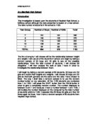
This investigation is based upon the students of Mayfield High School, a fictitious school although the data presented is based on a real school. The total number of students in the school is 1183.
Year Group
Number of Boys
Number of Girls
Total
7
51
31
282
8
45
25
270
9
18
43
261
0
06
94
200
1
84
86
70
TOTAL
604
579
183
The line of enquiry I will choose will be the relationship between height and weight; I will use all of the students in school and begin by taking a random sample of 30 boys and 30 girls to see all the possible relationships. From the total number of students, I will choose 60 altogether. I will then analyse the sets of data I have in order to investigate the relationship between them.
I will begin by taking a random sample of 60 students, 30 boys and 30 girls and record their heights and weights. I will choose 30 boys and 30 girls so that both genders are the same and the data I have chosen is fairer. The way I shall take a random sample is to use the random number button on my calculator. All the 1183 students are numbered from 1 to 1183. I will press the SHIFT button then the RAN# button in order to give a completely random number. The number displayed is between 0 and 1 and because I need a number between 1 and 1183, I will multiply the number displayed on the computer by the total number of students which is 1183. I repeated this 30 times for girls and then 30 times again for boys. Now I have a random sample of 60 students from Mayfield High School.
Random Sample
This is my random sample of boys and girls of Mayfield High School. I separated them into boys and girls so it is easier to analyse the data.
GIRLS
BOYS
Year
Height (m)
Weight (kg)
Year
Height (m)
Weight (kg)
7
.61
47
7
.47
41
7
.50
45
7
.64
50
7
.72
53
7
.36
45
7
.46
40
7
.71
49
7
.48
47
7
.65
64
7
.62
65
7
.51
59
7
.43
38
7
.60
43
7
.56
43
7
.62
47
8
.60
50
7
.51
39
8
.59
52
8
.70
49
8
.62
51
8
.56
59
8
.50
45
8
.52
45
8
.67
51
8
.66
43
9
.65
72
8
.65
51
9
.55
52
8
.55
68
9
.45
51
8
.60
38
9
.64
40
8
.53
32
9
.53
40
9
.70
47
9
.58
55
9
.56
60
9
.7
48
9
.69
65
9
.40
41
9
.64
35
9
.52
52
9
.56
53
0
.73
48
9
.71
44
0
.63
50
0
.63
44
0
.78
52
0
.83
75
0
.70
55
0
.74
56
1
.73
42
1
.88
75
1
.90
80
1
.79
72
1
.89
64
1
.62
54
1
2.00
86
1
.92
45
Now that I have my data I will put them into frequency/tally tables to make it easier to read and it is a better way to represent the data.
BOYS
Height (cm)
Tally
Frequency
30?h<140
I
40?h<150
I
50?h<160
IIIIIIII
8
60?h<170
IIIIIIIIIII
1
70?h<180
IIIIII
6
80?h<190
II
2
90?h<200
I
BOYS
Weight (kg)
Tally
Frequency
30?w<40
IIII
4
40?w<50
IIIIIIIIIIII
2
50?w<60
IIIIIII
7
60?w<70
IIII
4
70?w<80
III
3
80?w<90
0
GIRLS
Height (cm)
Tally
Frequency
30?h<140
0
40?h<150
IIIIII
6
50?h<160
IIIIIIII
8
60?h<170
IIIIIIII
8
70?h<180
IIIII
5
80?h<190
I
90?h<200
II
2
GIRLS
Weight (kg)
Tally
Frequency
30?w<40
I
40?w<50
IIIIIIIIIIII
2
50?w<60
IIIIIIIIIIII
2
60?w<70
II
2
70?w<80
I
80?w<90
II
2
Now I will record these results into different types of charts/diagrams to see the relationships between boys and girls and their heights and weights. I will first analyse the data I have by using a bar chart to compare the results I have between boys and girls.
Bar charts
Weight bar charts
Bar charts are a good way of analysing data as you can estimate the modal interval and the estimate the median interval. It is also one of the simplest ways of recording data.
This is a bar chart for the boys' weight.
This is a bar chart for the girls' weight.
> The evidence from these bar charts (sample) suggests that boys will tend to have roughly the same weight than girls. Although, in the group 50?w<60, nearly double the amount of girls had the weight frequency than the boys did. I think this is because the girls' weight is more condensed into to intervals of weight and boys tend to have a more spread out weight. My evidence also suggests that the boys' weight is more spread out than the girls' weight but my comments would me more accurate if the sample was extended.
Height bar charts
Now I will do the same for height. This is a bar chart for boys' height.
This is a bar chart for girls' height.
> The evidence from these bar charts suggests that boys have a higher height than girls and that the boys' height is more spread. I know that if I have a greater sample than my evidence will be clearer.
Mean, mode, median and range
I will now use estimate mean, mode, median and range to give me a more information and more clear evidence about weight and height. Firstly I will consider weight.
Mean weight
I will use my frequency tables to find out the mean of the weight for boys and girls.
BOYS
Weight (kg)
Tally
Frequency
Mid-point
fx
30?w<40
IIII
4
35
40
40?w<50
IIIIIIIIIIII
2
45
540
50?w<60
IIIIIII
7
55
385
60?w<70
IIII
4
65
260
70?w<80
III
3
75
225
80?w<90
0
85
0
TOTAL
30
550
Mean = 1550/30
Mean = 51.66
The mean weight for the boys is 51.66 kg.
GIRLS
Weight (kg)
Tally
Frequency
Mid-point
fx
30?w<40
I
35
35
40?w<50
IIIIIIIIIIII
2
45
540
50?w<60
IIIIIIIIIIIII
2
55
660
60?w<70
II
2
65
30
70?w<80
I
75
75
80?w<90
II
2
85
70
TOTAL
30
610
Mean = 1610/30
Mean = 53.66
The mean weight for the girls is 53.66 kg.
Modal weight
Boys weight
Stem
Leaf
Frequency
30
2,5,8,9
4
40
,3,3,4,4,5,5,5,7,7,9,9
2
50
0,1,3,4,6,9,9
7
60
0,4,5,8
4
70
2,5,5
3
80
0
Girls weight
Stem
Leaf
Frequency
30
8
40
0,0,0,0,1,2,3,5,5,7,7,8
2
50
0,0,1,1,1,2,2,2,2,3,5,5
2
60
4,5,
2
70
2
80
0,6
2
I can find the modal weight easily; I will just read it off my Stem and Leaf diagram which shows the most frequent value.
Modal weight for boys = 40?w<50
Modal weight for girls = 40?w<50, 50?w<60
Median weight
As there are 30 people in each sample, the median will be half way between the fifteenth and sixteenth values.
BOYS
GIRLS
Number
Weight (kg)
Weight (kg)
32
38
2
35
40
3
38
40
4
39
40
5
41
40
6
43
41
7
43
42
8
44
43
9
44
45
0
45
45
1
45
47
2
45
47
3
47
48
4
47
50
5
49
50
6
49
51
7
50
51
8
51
51
9
53
52
20
54
52
21
56
52
22
59
52
23
59
53
24
60
55
25
64
55
26
65
64
27
68
65
28
72
72
29
75
80
30
75
86
Median weight for boys = 49 kg
Median weight for girls = 50+51 = 50.5 =
51 kg 2
Range of weight
This shows me how spread my data for height is for girls and boys
Range of weight for boys = 75-32 = 43 kg
Range of weight for girls = 86-38 = 48 kg
I will now summarise my results into a clear table. The table shows the estimate mean, mode, median and range of boys and girls and I can easily see the differences.
Weight
Mean
Modal class interval
Median
Range
Boys
51.66
40?w<50
49
43
Girls
53.66
40?w<50, 50?w<60
51
48
> From this data I can see that girls have a slightly higher estimate mean, mode, and median. The range is also greater so this shows that the girls' sample is more spread than the boys and this could be a reason for my results. Although, I can see from my bar charts that a greater number of boys have small weights and a greater number of girls have larger weights, boys and girls will generally have the same weight when the mode is concerned.
> Evidence from the sample also suggests that 23 out of 30 boys, or 77% will have a weight between 40 and 70 and that 25 out of 30 girl's, or 83% will have a weight between 30 and 60. This also shows us that boys will tend to have a higher weight and girls will tend to have a lower weight.
Now I will consider the difference between the height of boys and girls.
Mean height
BOYS
Height (cm)
Tally
Frequency
Mid-point
Fx
30?h<140
I
35
35
40?h<150
I
45
45
50?h<160
IIIIIIII
8
55
240
60?h<170
IIIIIIIIIII
1
65
815
70?h<180
IIIIII
6
75
050
80?h<190
II
2
85
370
90?h<200
I
95
95
TOTAL
4950
I will use my frequency tables to find out the mean of the height for boys and girls.
Mean = 4950/30
Mean = 165
The mean height for boys is 165 cm.
GIRLS
Height (cm)
Tally
Frequency
Mid-point
fx
30?h<140
0
35
0
40?h<150
IIIIII
6
45
870
50?h<160
IIIIIIII
8
55
240
60?h<170
IIIIIIII
8
65
320
70?h<180
IIIII
5
75
875
80?h<190
I
85
85
90?h<200
II
2
95
390
TOTAL
4880
Mean = 4880/30
Mean = 162.66
The mean height for the girls is 162.66 cm.
Modal height
Boys' height
Stem
Leaf
Frequency
30
6
40
7
50
,1,2,3,5,6,6,6
8
60
0,0,2,2,3,4,4,5,5,6,9
1
70
0,0,1,1,4,9
6
80
3,8
2
90
2
200
0
Girls height
Stem
Leaf
Frequency
30
0
40
0,3,3,5,6,8
6
50
0,0,2,3,5,6,8,9
8
60
0,1,2,2,3,4,5,7
8
70
0,0,2,3,8
5
80
9
90
0
200
0
Once again, I can find the modal height easily; I will just read it off my stem and leaf diagrams, which has the most values.
Modal height for boys = 160?h<170
Modal weight for girls = 150?h<160, 160?h<170
Median height
BOYS
GIRLS
Number
Height (m)
Height (m)
.36
.4
2
.47
.43
3
.51
.43
4
.51
.45
5
.52
.46
6
.53
.48
7
.55
.50
8
.56
.50
9
.56
.52
0
.56
.53
1
.60
.55
2
.60
.56
3
.62
.58
4
.62
.59
5
.63
.60
6
.64
.61
7
.64
.62
8
.65
.62
9
.65
.63
20
.66
.64
21
.69
.65
22
.70
.67
Median height for boys = 163+164 = 163.5 = 164 cm 2
Median height for girls = 160+161 = 160.5
= 161 cm 2
Range of height
This shows me how spread my data for height is for girls and boys.
Range of height for boys = 192-136 = 56 cm
Range of height for girls = 200-140 = 60 cm
I will now summarise my results into a clear table. The table shows the estimate mean, mode, median and range of boys and girls and I can easily see the differences.
Height
Mean
Modal class interval
Median
Range
Boys
65
60?h<170
64
56
Girls
62.66
50?h<160, 160?h<170
61
60
> All of the measures of average (mean, mode and median) are greater for boys than for girls. The range of height is slightly greater for girls than boys. This could be a reason for the results. The mode was also close with the girls having the same amount of pupils in both 150?h<160, 160?h<170 intervals. Once again the results for boys and girls are quite close but more boys have a higher height than girls.
> So far from the evidence I found out, I can see that in my sample girls tend to have a slightly higher weight than boys. Also in my sample I can see that boys are slightly taller than girls and I can see that in my sample the data is more spread for girls than boys.
Histogram
As height and weight are continuous I can record them on a histogram. Histograms are a good, clear way to record data and they can also help me to find the modal interval and the mode.
...
This is a preview of the whole essay
> So far from the evidence I found out, I can see that in my sample girls tend to have a slightly higher weight than boys. Also in my sample I can see that boys are slightly taller than girls and I can see that in my sample the data is more spread for girls than boys.
Histogram
As height and weight are continuous I can record them on a histogram. Histograms are a good, clear way to record data and they can also help me to find the modal interval and the mode.
Weight
Since my class intervals are the same and that they are 10, I do not need to find the frequency density as if I multiply it by 10 I will get the same value as my frequency.
> From the histogram for boys' weight I can see that the modal interval is 40-50. The mode weight for boys is 46 kg. From the histogram for girls' weight the modal interval is 40-60. The mode weight for girls is 50 kg. I can see from this that girls have a higher weight than boys.
Height
From the histogram for boys' height I can see that the modal interval is 160-170 and the mode height is 164 cm. From the girls' histogram I can see the modal interval is 150-170 and the mode height is 160 cm. I can see that boys have a slightly higher height than girls.
Frequency polygons
Frequency polygons are a good way to compare my two sets of continuous data. By using frequency polygons I can compare boys and girls height and weight.
Height
This frequency polygon shows us that boys have a higher height than girls.
Weight
This frequency polygon shows us that girls have a slightly higher weight than boys but they are both close.
> As I said earlier, in weight all three measures of average showed that girls have a slightly higher estimate mean, mode, and median. The results are very close together and the range is also greater so this shows that the girls sample is more spread than the boys and this could be a reason for my results. Evidence from the sample also suggests that 23 out of 30 boys, or 77% will have a weight between 40 and 70 and those 25 out of 30 girls, or 83% will have a weight between 30 and 60. The frequency polygons show that there are fewer boys with smaller weight and they also show that most boys and girls have the same weight.
> In height boys were generally taller with the measures of average being higher than girls. Also, evidence from the sample shows that 20 out of 30 boys, or 67% had heights higher than 160 cm whilst 16 out of 30, or 53% girls had a height higher than 160 cm. The frequency polygon also shows more boys have higher heights than girls.
> These conclusions are based on a sample of only 30 boys and 30 girls. If I was to increase the sample or repeat the whole exercise again I could confirm my results.
I will now test the following hypothesis:
> In general the taller a person is, the more they will weigh.
To test this hypothesis I will take a new random sample of 30 students.
Height (m)
Weight (kg)
Height (m)
Weight (kg)
.60
50
.53
65
.73
51
.6
48
.49
40
.57
40
.36
44
.56
50
.47
38
.65
48
.51
38
.47
56
.54
42
.64
42
.48
40
.75
56
.42
52
.67
66
.58
52
.60
56
.56
45
.52
60
.70
58
.72
56
.52
45
.8
60
.62
52
.75
57
.8
60
.65
55
.55
36
.60
66
Scatter diagram
I will now draw a scatter diagram for this data to compare height and weight.
> My line of best fit must have passed through the point (160, 50). I worked this out by finding the mean of the X and Y axis and then saw were they crossed. There is a positive correlation between height and weight. This suggests the taller the person the more they will weigh.
> The line of best fit suggests that somebody with a weight of 55 kg will have a height of 170 cm.
> Height and weight are also affected by gender. Earlier in this investigation, I found out that boys tend to be taller. I will now see what the correlation will be if boys and girls were to be considered separately using my original sample.
> There is a stronger correlation between height and weight if boys and girls were to be considered separately. The lines of best fit on my diagrams predict that a girl with a weight of 60 kg would have a height of 1.76 m, whereas a boy with the same weight would have a height of 1.85 m. This tells me that boys have smaller weights than girls. Although, a girl with the weight of 40 kg would have a height of 1.42 m, a boy would have the height of 137 cm. This tells me that girls with smaller weights are taller than boys. There is also a stronger correlation on the scatter diagram for girls.
I can also use the formula for the line of best fit to predict student's weights or heights:
Boys only: y = 39.23x - 12.652
Girls only: y = 59.706x - 44.838
Mixed sample: y = 50.967x - 31.297
For example, to predict the weight of a girl with the height of 1.50 m:
y = 59.706x - 44.838
So y = (59.706 X 1.50) - 44.838
= 44.721
Using the equation of my line of best fit for girls, I can predict that a girl with the height of 1.50 m will have a weight of 44.72 kg.
Predict the height of a boy with the weight of 60 kg.
y = 39.23 - 12.652
So x = y + 12.652
39.23
If y = 60 then
x = 60 + 12.652 = 1.85 (2 d.p)
39.23
Using the equation of my line of best fit for boys, I can predict that a boy with the weight of 60 kg will be 1.85 m tall. If I look on my scatter diagrams I can see that these two predictions are correct.
> The line of best fit is a best estimation of relationship between height and weight. There are exceptional values in my data, such as the boy with a weight of 45 kg who is 1.92 m tall, which fall outside the general trend. The line of best fit is a continuous relationship. These values could be a result of puberty, which takes place around year 9 and year 10, were some students might gain height, weight or both.
Cumulative frequency
Firstly, I will draw a cumulative frequency curve for weight, then for height.
Cumulative frequency table for weight.
Weight
Cumulative frequency
Boys
Girls
Mixed
<40
4
5
<50
6
3
9
<60
23
25
48
<70
27
27
54
<80
30
28
58
<90
30
30
60
Cumulative frequency table for height.
Height
Cumulative frequency
Boys
Girls
Mixed
<140
0
<150
2
6
8
<160
0
4
24
<170
21
22
43
<180
27
27
54
<190
29
28
57
<200
30
30
60
> A reason for drawing cumulative frequency curves for continuous variables like height and weight is that I can easily read off the median, upper quartile, lower quartile and the interquartile range. I will put them into a table for both height and weight.
Weight
Median
Lower quartile
Upper quartile
Interquartile range
Mixed
55
47
59
2
Boys
50
43.5
60
6.5
Girls
52
46
57
1
Height
Median
Lower quartile
Upper quartile
Interquartile range
Mixed
62
55
71
6
Boys
64
57.5
72
4.5
Girls
62
52
70
8
> My data implies that if we select a boy from random from the school, the probability that he will have a height between 150 and 170 will be 0.63. I can estimate that 63% of boys in the school will be between 150 cm and 170 cm. If I was to select a girl from random, the probability that she will also have a height between 150 cm and 170 cm will be 0.53.
I will now draw box and whisker diagrams to show the median, upper quartile, lower quartile and the minimum and maximum values.
> The box and whisker diagrams show that the interquartile range for boys is only 0.4 cm greater than girls. This suggests that the boys' heights and girls' heights are closely spread out; there is not a big difference between them. There is not much of a difference if they are considered mixed either.
> The box and whisker diagram for weight shows us the same difference between boys and girls (both are spread out in roughly the same way). Although when considered mixed the data is more spread out.
> Whilst in general boys are taller than girls, the evidence suggests that 7 out of 30 or 23% of girls have a higher height than the upper quartile height of boys. Also, in general girls' weigh more than boys there is evidence that suggests that 23% of boys have a higher weight than girls above 60 kg.
Standard deviation
Standard deviation will help me find out how my data is spread out around the mean. Firstly I will calculate the standard deviation of boys' height.
µ = mean
n = number of values (30)
I will be using this formula to find the standard deviation:
Standard deviation = V?x² - µ²
n
Boys Weight
x
x²
41
681
50
2500
45
2025
49
2401
64
4096
59
3481
43
849
47
2209
39
521
49
2401
59
3481
45
2025
43
849
51
2601
68
4624
38
444
32
024
47
2209
60
3600
65
4225
35
225
53
2809
44
936
44
936
75
5625
56
3136
75
5625
72
5184
54
2916
45
2025
547
83663
µ = 51.56667
Standard deviation = V83663 - 51.56667²
30
Standard deviation = 11.386 (3 d.p)
From this evidence I can see that the mean for boys' weight is not a realistic way of interpreting the data and the mean is unreliable.
Boys Height
x
x²
47
21609
64
26896
36
8496
71
29241
65
27225
51
22801
60
25600
62
26244
51
22801
70
28900
56
24336
52
23104
66
27556
65
27225
55
24025
60
25600
53
23409
70
28900
56
24336
69
28561
64
26896
56
24336
71
29241
63
26569
83
33489
74
30276
88
35344
79
32041
62
26244
92
36864
4911
808165
µ = 163.7
Standard deviation = V808165 - 163.7²
30
Standard deviation = 11.88 (2 d.p)
I can see that my mean for boys' height isn't a good way to judge my data. It is unreliable as the standard deviation is quite high.
Girls Weight
x
x²
47
2209
45
2025
53
2809
40
600
47
2209
65
4225
38
444
43
849
50
2500
52
2704
51
2601
45
2025
40
600
51
2601
72
5184
52
2704
51
2601
40
600
40
600
55
3025
48
2304
41
681
52
2704
50
2500
52
2704
55
3025
42
764
80
6400
64
4096
86
7396
547
83689
µ = 51.56667
Standard deviation = V83689 - 51.56667²
30
Standard deviation = 10.963 (3 d.p)
From the outcome of the standard deviation for girls' weight, I can see that the mean for the girls' weight isn't a good way to interpret the data. The mean is unreliable.
Girls Height
x
x²
61
25921
50
22500
72
29584
46
21316
48
21904
62
26244
43
20449
56
24336
60
25600
59
25281
62
26244
50
22500
43
20449
67
27889
65
27225
55
24025
45
21025
64
26896
53
23409
58
24964
70
28900
40
9600
52
23104
63
26569
78
31684
70
28900
73
29929
90
36100
89
35721
200
40000
4844
788268
µ = 161.4667
Standard deviation = V788268 - 161.4667²
30
Standard deviation = 14.287 (3 d.p)
The standard deviation for girls' height is high and therefore I can not use the mean to judge my data. The mean is unreliable.
> From the results I have got for standard deviation I can see that the mean for girls and boy's weights and heights isn't a reliable way to interpret the data I have collected.
Product-moment correlation coefficient r (PMCC)
The product moment correlation coefficient is good for seeing how strong the correlations are on my scatter graphs. I can predict that the correlation for girls will be stronger than that for boys.
Formula: r = Sxy
V (SxxSyy)
Sxy = ?xy - ?x?y
n
Sxx = ?x² - (?x) ²
n
Syy = ?y² - (?y) ²
n
PMCC for boys
x
y
x²
y²
xy
.47
41
2.1609
681
60.27
.64
50
2.6896
2500
82
.36
45
.8496
2025
61.2
.71
49
2.9241
2401
83.79
.65
64
2.7225
4096
05.6
.51
59
2.2801
3481
89.09
.60
43
2.56
849
68.8
.62
47
2.6244
2209
76.14
.51
39
2.2801
521
58.89
.70
49
2.89
2401
83.3
.56
59
2.4336
3481
92.04
.52
45
2.3104
2025
68.4
.66
43
2.7556
849
71.38
.65
51
2.7225
2601
84.15
.55
68
2.4025
4624
05.4
.60
38
2.56
444
60.8
.53
32
2.3409
024
48.96
.70
47
2.89
2209
79.9
.56
60
2.4336
3600
93.6
.69
65
2.8561
4225
09.85
.64
35
2.6896
225
57.4
.56
53
2.4336
2809
82.68
.71
44
2.9241
936
75.24
.63
44
2.6569
936
71.72
.83
75
3.3489
5625
37.25
.74
56
3.0276
3136
97.44
.88
75
3.5344
5625
41
.79
72
3.2041
5184
28.88
.62
54
2.6244
2916
87.48
.92
45
3.6864
2025
86.4
49.11
547
80.8165
83663
2549.05
r = (2549.05) - (49.11X1547)
30 .
V (80.8165) - (49.11)² X (83663) - (1547) ²
30 30
r = 16.611
40.58170188
r = 0.409332
> I can see from calculating the PMCC, that my strength for the correlation between the two variables, height and weight, for boys is weak.
PMCC for girls
x
y
x²
y²
xy
.61
47
2.5921
2209
75.67
.50
45
2.25
2025
67.5
.72
53
2.9584
2809
91.16
.46
40
2.1316
600
58.4
.48
47
2.1904
2209
69.56
.62
65
2.6244
4225
05.3
.43
38
2.0449
444
54.34
.56
43
2.4336
849
67.08
.60
50
2.56
2500
80
.59
52
2.5281
2704
82.68
.62
51
2.6244
2601
82.62
.50
45
2.25
2025
67.5
.43
40
2.0449
600
57.2
.67
51
2.7889
2601
85.17
.65
72
2.7225
5184
18.8
.55
52
2.4025
2704
80.6
.45
51
2.1025
2601
73.95
.64
40
2.6896
600
65.6
.53
40
2.3409
600
61.2
.58
55
2.4964
3025
86.9
.7
48
2.89
2304
81.6
.4
41
.96
681
57.4
.52
52
2.3104
2704
79.04
.63
50
2.6569
2500
81.5
.78
52
3.1684
2704
92.56
.70
55
2.89
3025
93.5
.73
42
2.9929
764
72.66
.90
80
3.61
6400
52
.89
64
3.5721
4096
20.96
2.00
86
4
7396
72
48.44
547
78.8268
83689
2534.45
r = (2534.45) - (48.44X1547)
30 .
V (78.8268) - (48.44)² X (83689) - (1547) ²
30 30
r = 36.56066667
48.96490299
r = 0.74667
> I can see from the answer that my prediction was right. The correlation for girls' height and weight is definitely stronger than that for boys. This tells me that there is a better relationship between height and weight for girls more than boys.
Conclusion from random sampling
> There is a positive correlation between height and weight. In general tall people will weigh more than smaller people.
> The points on the scatter diagram for the girls are less dispersed about the line of best fit than those for boys. This suggests that the correlation is better for girls than for boys.
> The points on the scatter diagrams for boys and girls are less dispersed than the points on the scatter diagram for mixed sample of boys and girls. This suggests that the correlation between height and weight is better when girls and boys are considered separately.
> I can use the scatter diagrams to give reasonable estimates of height and weight. This can be done either by reading from the graph or using the equations for the line of best fit.
> The cumulative frequency curves confirm that boys and girls have quite a close height and weight, with girls being slightly higher in weight and boys slightly higher in height.
> The median for boys is higher in height and the median for girls is higher in weight.
> From the box and whisker diagrams I can conclude that, in general boys are taller than girls, but not exclusively so. The cumulative frequency curves can be used to estimate that 23% of girls have a higher height than 172 cm, the upper quartile height of boys.
> Also from the box and whisker diagrams I can conclude that in general girls weigh more than boys but not exclusively so. The cumulative frequency curves can be used to estimate that 23% of boys have a higher weight than girls above 60 kg. This could also be a result of my sampling which has more students from year 7 and 8 then 9, 10 or 11. This could mean more lighter people than heavier people
> I could have had a greater confidence in these results if we had taken larger samples. Also, my predictions are based on general trends observed in the data. In both samples there were exceptional individuals whose results fell outside the general trend.
> When age is taken to consideration, the correlation between height and weight will be better than when age is not considered.
This was based upon 60 students sampled at random. To ensure that the students from different age groups are represented equally I will now take a stratified sample.
Stratified Sample
Year Group
Number of Boys
Number of Girls
Total
7
51
31
282
8
45
25
270
9
18
43
261
0
06
94
200
1
84
86
70
TOTAL
604
579
183
I will use this information to find the Stratified sample of 30 boys and 30 girls, so a total of 60 pupils. I will use 60 pupils again as it will provide more accurate results. I will divide the amount of boys and girls in each year by the total amount of pupils (1183) and then multiply that number by the amount of random sampled pupils I will take (60).
Boys
total people In school
boys/total
X 60
51
183
0.127642
7.658495
45
183
0.12257
7.354184
18
183
0.099746
5.984784
06
183
0.089603
5.376162
84
183
0.071006
4.260355
Girls
total people In school
girls/total
X 60
31
183
0.110735
6.644125
25
183
0.105664
6.339814
43
183
0.120879
7.252747
94
183
0.079459
4.76754
86
183
0.072697
4.361792
total
total people In school
total/total
X 60
282
183
0.238377
4.30262
270
183
0.228233
3.694
261
183
0.220626
3.23753
200
183
0.169062
0.1437
70
183
0.143702
8.622147
By taking a stratified sample I can be sure as possible that my sample is representative of the whole school. As far as possible, my sample is free from bias caused by gender or age divisions.
Year group
Number of boys
Number of girls
Total
7
8
7
5
8
7
7
4
9
6
7
3
0
5
5
0
1
4
4
8
TOTAL
30
30
60
I will now use the SHIFT RAN# button on my calculator to pick the right amount of boys and girls in each year to give the following results.
MALE
FEMALE
Year
Height (cm)
Weight (kg)
Year
Height (m)
Weight (kg)
7
.48
44
7
.61
52
7
.55
53
7
.56
45
7
.62
48
7
.62
50
7
.60
40
7
.52
40
7
.49
38
7
.42
41
7
.59
45
7
.52
33
7
.45
40
7
.42
30
7
.50
41
8
.62
54
8
.77
54
8
.65
52
8
.70
49
8
.73
44
8
.52
52
8
.55
57
8
.50
41
8
.58
52
8
.72
51
8
.56
45
8
.67
52
8
.70
58
8
.65
35
9
.52
50
9
.60
60
9
.68
47
9
.56
60
9
.56
50
9
.66
54
9
.65
48
9
.66
70
9
.47
56
9
.52
52
9
.64
42
9
.75
75
9
.75
56
0
.75
45
0
.63
50
0
.83
60
0
.80
62
0
.80
60
0
.80
68
0
.71
57
0
.69
50
0
.66
66
0
.80
74
1
.63
60
1
.60
55
1
.67
52
1
.52
48
1
.80
49
1
.57
54
1
.66
70
1
.39
42
Now that I have my data I will put them into frequency/tally tables to make it easier to read and it is a better way to represent the data.
BOYS
Height (cm)
Tally
Frequency
30?h<140
0
40?h<150
III
3
50?h<160
IIIIIII
7
60?h<170
IIIIIIIIIII
1
70?h<180
IIIIII
6
80?h<190
III
3
90?h<200
0
TOTAL
30
BOYS
Weight (kg)
Tally
Boys frequency
30?w<40
II
2
40?w<50
IIIIIIIIII
0
50?w<60
IIIIIIIII
9
60?w<70
IIIIII
6
70?w<80
III
3
80?w<90
0
TOTAL
30
GIRLS
Height (cm)
Tally
Frequency
30?h<140
I
40?h<150
III
3
50?h<160
IIIIIIIIII
0
60?h<170
IIIIIIIIIII
0
70?h<180
III
3
80?h<190
III
3
90?h<200
0
TOTAL
30
GIRLS
Weight (kg)
Tally
Girls frequency
30?w<40
II
2
40?w<50
IIIIIIIIII
0
50?w<60
IIIIIIIIIIIIIII
5
60?w<70
II
2
70?w<80
I
80?w<90
0
TOTAL
30
Now I will repeat what I did for normal random sampling but this time for stratified sampling and I will then compare the results.
Mean, mode, median and range
I will now use estimate mean, mode, median and range to give me a more information and more clear evidence about weight and height. Firstly I will consider weight.
Mean weight
BOYS
Weight (kg)
Tally
Boys frequency
Mid-point
fx
30?w<40
II
2
35
70
40?w<50
IIIIIIIIII
0
45
450
50?w<60
IIIIIIIII
9
55
495
60?w<70
IIIIII
6
65
390
70?w<80
III
3
75
225
80?w<90
I
0
85
0
TOTAL
30
630
Mean = 1630/30
Mean = 54.33
The mean weight for boys is 54.33 kg.
GIRLS
Weight (kg)
Tally
Girls frequency
Mid-point
fx
30?w<40
II
2
35
70
40?w<50
IIIIIIIIII
0
45
450
50?w<60
IIIIIIIIIIIIIII
5
55
825
60?w<70
II
2
65
30
70?w<80
I
75
75
80?w<90
I
0
85
0
TOTAL
30
550
Mean = 1550/30
Mean = 51.667
The mean weight for girls is 51.667 kg.
Modal weight
Boys
Stem
Leaf
Frequency
30
5,8
2
40
0,0,1,1,4,5,5,8,9,9
0
50
,2,2,2,2,3,4,4,7
9
60
0,0,0,0,0,6
6
70
0,0,5
3
80
Girls
Stem
Leaf
Frequency
30
0,3
2
40
0,1,2,2,4,5,5,7,8,8,
0
50
0,0,0,0,0,2,2,2,4,4,5,6,6,7,8
5
60
2,8
2
70
4
80
Modal weight for boys = 40?w<50
Modal weight for girls = 50?w<60
Median weight
I can also read the median weight from my stem and leaf diagrams, it between the 15th and 16th values.
Median weight for boys = 52 kg
Median weight for girls = 50 kg
Range of weight
This shows me how spread my data for height is for girls and boys I will take away the lowest value from the highest.
Range of weight for boys = 75-35 = 40 kg
Range of weight for girls = 74-33 = 41 kg
I will now summarise my results into a clear table. The table shows the estimate mean, mode, median and range of boys and girls and I can easily see the differences.
Weight
Mean
Mode
Median
Range
Boys
54.33
40?w<50
52
40
Girls
51.66
50?w<60
50
41
> This shows some differences from the random sample. The mean and median is higher for boys although the mode is higher for girls. The range is almost the same so it doesn't really affect the results. This tells me boys' weight would be higher.
Now I will find the mean, mode, median for height.
Mean height
BOYS
Height (cm)
Tally
Frequency
Mid-point
fx
30?h<140
I
0
35
0
40?h<150
III
3
45
435
50?h<160
IIIIIII
7
55
085
60?h<170
IIIIIIIIIII
1
65
815
70?h<180
IIIIII
6
75
050
80?h<190
III
3
85
555
90?h<200
I
0
95
0
TOTAL
30
4940
Mean = 4940/30
Mean = 164.66
The mean height for boys = 164.66 cm
GIRLS
Height (cm)
Tally
Frequency
Mid-point
fx
30?h<140
I
35
35
40?h<150
III
3
45
435
50?h<160
IIIIIIIIII
0
55
550
60?h<170
IIIIIIIIIII
0
65
650
70?h<180
III
3
75
525
80?h<190
III
3
85
555
90?h<200
I
0
95
0
TOTAL
30
4850
Mean = 4850/30
Mean = 161.66
The mean height for girls = 161.66 cm
Modal height
Boys
Stem
Leaf
Frequency
30
0
40
5,8,9
3
50
0,0,2,2,5,6,9
7
60
0,0,2,3,5,6,6,6,6,7,7
1
70
0,1,2,5,5,7,
6
80
0,0,3
3
90
0
Girls
Stem
Leaf
Frequency
30
9
40
2,2,7
3
50
2,2,2,2,5,6,6,6,7,8
0
60
0,1,2,2,3,4,5,5,8,9
0
70
0,3,5
3
80
0,0,0
3
90
Modal height for boys = 160?h<170
Modal weight for girls = 150?h<160, 160?h<170
Median height
I can also read the median height from my stem and leaf diagrams, it between the 15th and 16th values.
Median height for boys = 156 cm
Median height for girls = 161 cm
Range of height
Range of height for boys = 183-145 = 38 cm
Range of height for girls = 180-139 = 41 cm
I will now summarise my results into a clear table. The table shows the estimate mean, mode, median and range of boys and girls and I can easily see the differences.
Height
Mean
Mode
Median
Range
Boys
64.66
60?h<170
56
38
Girls
61.66
50?h<160, 160?h<170
61
41
> The mean for height is higher for boys than girls and this tells me that boys' height is higher than girls in general. The mode for both girls and boys are close together although the girls' median height is higher. The mode was also close with the girls having the same amount of pupils in both 150?h<160, 160?h<170 intervals. Once again the results for boys and girls are quite close but more boys have a higher height than girls.
> So far from the evidence I found out, I can see that in my sample boys tend to have a slightly higher weight and height than girls. Also I can see that in my sample the data is more spread for girls than boys.
Histogram
As height and weight are continuous I can record them on a histogram. Histograms are a good, clear way to record data and they can also help me to find the modal interval and the mode. As my class widths are the same the frequency density will be the same as the frequency.
Height
Since my class intervals are the same and that they are 10, I do not need to find the frequency density as if I multiply it by 10 I will get the same value as my frequency.
> From the histogram for boys' weight I can see that the modal interval is 40-50. The mode weight for boys is 49 kg. From the histogram for girls' weight the modal interval is 50-60. The mode weight for girls is 53 kg. I can see from this that more girls have a lower weight than boys.
Weight
From the histogram for boys' height I can see that the modal interval is 160-170 and the mode height is 164.5 cm. From the girls' histogram I can see the modal interval is 150-170 and the mode height is 160 cm. I can see that boys have a higher height than girls.
Frequency polygon
Frequency polygons are a good way to compare my two sets of continuous data. By using frequency polygons I can compare boys and girls height and weight.
Height
The frequency polygon for height shows us that boys' height is more evenly spread out and that boys are taller.
Weight
The frequency polygon for weight shows us that, once again boys' weight is more evenly spread and more girls have a weight between 50 and 60. It also tells us that boys tend to weigh more than girls.
> In weight, two measures of average showed that boys have a slightly higher estimate mean and median. The mode for weight is greater for girls, which tells me more girls have lower weights than higher weights. The results are very close together and the range is also close so this shows that both samples are evenly spread. More girls will have lower weights than boys and therefore boys will weigh more. Evidence from the sample suggests that 27 out of 30 girls or 90% will have a weight lower than 60 kg whilst 21 out of 30 boys or 70% will have a weight lower than 60 kg. The frequency polygons show that there are fewer boys with smaller weight and they also show that most boys and girls have the same weight.
> In height boys were generally taller with the measures of average being higher than girls in mean and mode. This tells me boys are taller than girls. Also, evidence from the sample shows that 20 out of 30 boys or 67% had heights higher than 160 cm whilst 16 out of 30, or 53% girls had a height higher than 160 cm. This tells me that more boys are taller than girls. The frequency polygon also shows more boys have higher heights than girls.
> These conclusions are based on a sample of only 30 boys and 30 girls. If I was to increase the sample or repeat the whole exercise again I could confirm my results.
Once again, I will now test the following hypothesis:
> In general the taller a person is, the more they will weigh.
Scatter diagram
To test this hypothesis I will draw scatter diagrams to give a clear representation of the relationship between height and weight.
> My line of best fit must have passed through the point (160, 50) for mixed population. I worked this out by finding the mean of the X and Y axis and then saw were they crossed. There is a positive correlation between height and weight. This suggests the taller the person the more they will weigh.
> There is a stronger correlation between height and weight if boys and girls were to be considered separately. The lines of best fit on my diagrams predict that a girl with a weight of 60 kg would have a height of 1.78 m, whereas a boy with the same weight would have a height of 1.81 m. This tells me that boys are taller than girls. Although, a girl with the weight of 40 kg would have a height of 1.42 m whilst a boy would have the height of 1.38 m. This tells me that girls with smaller weights are taller than boys. There is also a stronger correlation on the scatter diagram for girls.
I can also use the formula for the line of best fit to predict student's weights or heights:
Boys only: y = 43.481x - 18.687
Girls only: y = 55.633x - 39.088
Mixed sample: y = 50.335x - 30.243
For example, to predict the weight of a girl with the height of 1.50 m:
y = 55.633x - 39.088
So y = (55.633 X 1.50) - 39.088
= 44.441
Using the equation of my line of best fit for girls, I can predict that a girl with the height of 1.50 m will have a weight of 44.441 kg.
Predict the height of a boy with the weight of 60 kg.
y = 43.481x - 18.687
So x = y + 18.687
43.481
If y = 60 then
x = 60 + 18.687 = 1.81 (2 d.p)
43.481
Using the equation of my line of best fit for boys, I can predict that a boy with the weight of 60 kg will be 1.85 m tall. If I look on my scatter diagrams I can see that these two predictions are correct.
> The line of best fit is a best estimation of relationship between height and weight. There are exceptional values in my data, such as the boy with a weight of 45 kg who is 1.75 m tall, which fall outside the general trend. The line of best fit is a continuous relationship. These values could be a result of puberty, which takes place around year 9 and year 10, were some students might gain height, weight or both.
Cumulative frequency
Firstly, I will draw a cumulative frequency curve for weight, then for height. It makes comparing the data much easier.
Cumulative frequency table for weight.
Weight
Cumulative frequency
Girls
Boys
Mixed
<40
2
2
4
<50
2
2
24
<60
27
21
48
<70
29
27
56
<80
30
30
60
<90
30
30
60
Height
Cumulative frequency
Girls
Boys
Mixed
<140
0
<150
4
3
7
<160
4
0
24
<170
24
21
45
<180
27
27
54
<190
30
30
60
<200
30
30
60
Cumulative frequency table for height.
> A reason for drawing cumulative frequency curves for continuous variables like height and weight is that I can easily read off the median, upper quartile, lower quartile and the interquartile range. I will put them into a table for both height and weight.
Weight
Median
Lower quartile
Upper quartile
Interquartile range
Mixed
52
47
58
1
Boys
54
46
62
6
Girls
53
46
57
1
Height
Median
Lower quartile
Upper quartile
Interquartile range
Mixed
63
55
70
5
Boys
64
56
72
6
Girls
61
55
68
3
> My data implies that if we select a boy from random from the school, the probability that he will have a height between 160 and 180 will be 0.56. I can estimate that 56% of boys in the school will be between 150 cm and 170 cm. If I was to select a girl from random, the probability that she will also have a height between 160 cm and 180 cm will be 0.43.
> My data implies that if we select a boy from random from the school, the probability that he will have a weight between 60 and 90 will be 0.3. I can estimate that 30% of boys in the school will be between 60 kg and 90 kg. If I was to select a girl from random, the probability that she will also have a height between 60 kg and 90 kg will be 0.1. I can estimate that 10% of girls in the school will weigh between 60 kg and 90 kg.
I will now draw box and whisker diagrams to show the median, upper quartile, lower quartile and the minimum and maximum values.
> The box and whisker diagrams show that the interquartile range for boys is greater than girls. This suggests that the boys' height is more spread out than girls' heights and boys are generally taller than girls. There is not much of a difference if they are considered mixed either.
> The box and whisker diagram for weight shows us the same difference between boys and girls (boys generally weigh more). Also, the data is clearer if age is considered separately.
> Whilst in general boys are taller than girls, the evidence suggests that out of 30 or 20% of girls have a higher height than the upper quartile height of boys. Also, in general boys weigh more than girls there is evidence that suggests that 10% of girls have a higher weight than boys above 60 kg.
Standard deviation
Standard deviation will help me find out how my data is spread out around the mean. Firstly I will calculate the standard deviation of boys' height.
µ = mean
n = number of values (30)
I will be using this formula to find the standard deviation:
Standard deviation = V?x² - µ²
n
Boys Weight
x
x²
44
936
53
2809
48
2304
40
600
38
444
45
2025
40
600
41
681
54
2916
49
2401
52
2704
41
681
51
2601
52
2704
35
225
60
3600
60
3600
54
2916
70
4900
52
2704
75
5625
45
2025
60
3600
60
3600
57
3249
66
4356
60
3600
52
2704
49
2401
70
4900
573
85411
µ = 52.43333
Standard deviation = V85411 - 52.43333²
30
Standard deviation = 9.888 (3 d.p)
From this evidence I can see that the mean for boys' weight is not a realistic way of interpreting the data and the mean is unreliable.
Boys Height
x
x²
48
21904
55
24025
62
26244
60
25600
49
22201
59
25281
45
21025
50
22500
77
31329
70
28900
52
23104
50
22500
72
29584
67
27889
65
27225
60
25600
56
24336
66
27556
66
27556
52
23104
75
30625
75
30625
83
33489
80
32400
71
29241
66
27556
63
26569
67
27889
80
32400
66
27556
4907
805813
µ = 163.5667
Standard deviation = V805813 - 163.5667²
30
Standard deviation = 10.313 (3 d.p)
I can see that my mean for boys' height isn't a good way to judge my data. It is unreliable as the standard deviation is quite high.
Girls Weight
x
x²
52
2704
45
2025
50
2500
40
600
41
681
33
089
30
900
54
2916
52
2704
44
936
57
3249
52
2704
45
2025
58
3364
50
2500
47
2209
50
2500
48
2304
56
3136
42
764
56
3136
50
2500
62
3844
68
4624
50
2500
74
5476
55
3025
48
2304
54
2916
42
764
505
77899
µ = 50.16667
Standard deviation = V77899 - 50.16667²
30
Standard deviation = 8.941 (3 d.p)
From the outcome of the standard deviation for girls' weight, I can see that the mean for the girls' weight isn't a good way to interpret the data. The mean is unreliable.
Girls Height
x
x²
61
25921
56
24336
62
26244
52
23104
42
20164
52
23104
42
20164
62
26244
65
27225
73
29929
55
24025
58
24964
56
24336
70
28900
52
23104
68
28224
56
24336
65
27225
47
21609
64
26896
75
30625
63
26569
80
32400
80
32400
69
28561
80
32400
60
25600
52
23104
57
24649
39
9321
4813
775683
µ = 160.4333
Standard deviation = V775683 - 160.4333²
30
Standard deviation = 10.828 (3 d.p)
The standard deviation for girls' height is high and therefore I can not use the mean to judge my data. The mean is unreliable.
> From the results I have got for standard deviation I can see that the mean for girls and boy's weights and heights isn't a reliable way to interpret the data I have collected. Although, the standard deviation results I have got are better than the ones I got from random sampling.
Product-moment correlation coefficient r (PMCC)
The product moment correlation coefficient is good for seeing how strong the correlations are on my scatter graphs. I can predict that the correlation for girls will be stronger than that for boys.
Formula: r = Sxy
V (SxxSyy)
Sxy = ?xy - ?x?y
n
Sxx = ?x² - (?x) ²
n
Syy = ?y² - (?y) ²
n
PMCC for boys
x
y
x²
y²
xy
.48
44
2.1904
936
65.12
.55
53
2.4025
2809
82.15
.62
48
2.6244
2304
77.76
.60
40
2.56
600
64
.49
38
2.2201
444
56.62
.59
45
2.5281
2025
71.55
.45
40
2.1025
600
58
.50
41
2.25
681
61.5
.77
54
3.1329
2916
95.58
.70
49
2.89
2401
83.3
.52
52
2.3104
2704
79.04
.50
41
2.25
681
61.5
.72
51
2.9584
2601
87.72
.67
52
2.7889
2704
86.84
.65
35
2.7225
225
57.75
.60
60
2.56
3600
96
.56
60
2.4336
3600
93.6
.66
54
2.7556
2916
89.64
.66
70
2.7556
4900
16.2
.52
52
2.3104
2704
79.04
.75
75
3.0625
5625
31.25
.75
45
3.0625
2025
78.75
.83
60
3.3489
3600
09.8
.80
60
3.24
3600
08
.71
57
2.9241
3249
97.47
.66
66
2.7556
4356
09.56
.63
60
2.6569
3600
97.8
.67
52
2.7889
2704
86.84
.80
49
3.24
2401
88.2
.66
70
2.7556
4900
16.2
49.07
573
80.5813
85411
2586.78
r = (2586.78) - (49.07 X 1573)
30 .
V (80.5813) - (49.07)² X (85411) - (1573) ²
30 30
r = 13.87633333
30.59648441
r = 0.45352705
> I can see from calculating the PMCC, that my strength for the correlation between the two variables, height and weight, for boys is quite weak.
PMCC for girls
x
y
x²
y²
xy
.61
52
2.5921
2704
83.72
.56
45
2.4336
2025
70.2
.62
50
2.6244
2500
81
.52
40
2.3104
600
60.8
.42
41
2.0164
681
58.22
.52
33
2.3104
089
50.16
.42
30
2.0164
900
42.6
.62
54
2.6244
2916
87.48
.65
52
2.7225
2704
85.8
.73
44
2.9929
936
76.12
.55
57
2.4025
3249
88.35
.58
52
2.4964
2704
82.16
.56
45
2.4336
2025
70.2
.70
58
2.89
3364
98.6
.52
50
2.3104
2500
76
.68
47
2.8224
2209
78.96
.56
50
2.4336
2500
78
.65
48
2.7225
2304
79.2
.47
56
2.1609
3136
82.32
.64
42
2.6896
764
68.88
.75
56
3.0625
3136
98
.63
50
2.6569
2500
81.5
.8
62
3.24
3844
11.6
.80
68
3.24
4624
22.4
.69
50
2.8561
2500
84.5
.80
74
3.24
5476
33.2
.60
55
2.56
3025
88
.52
48
2.3104
2304
72.96
.57
54
2.4649
2916
84.78
.39
42
.9321
764
58.38
48.13
505
77.5683
77899
2434.09
r = (2434.09) - (48.13 X 1505)
30 .
V (77.5683) - (48.13)² X (77899) - (1505) ²
30 30
r = 19.56833333
29.04346997
r = 0.673760172
> I can see from the answer that my prediction was right. The correlation for girls' height and weight is definitely stronger than that for boys. This tells me that there is a better relationship between height and weight for girls more than boys.
This scatter diagram for boys has a weak correlation.
This scatter diagram for girls has a strong correlation.
Conclusion from stratified sampling
> The results from doing histograms, frequency polygons etc. proved that the results were more accurate and made more sense than that from the random sampling.
> There is a positive correlation between height and weight. In general tall people will weigh more than smaller people.
> Also, in general boys tend to weigh more and be taller then girls.
> By doing stratified sampling, there were a fewer exceptional values caused by different year groups and therefore ages. This made by results more accurate so I will use these results to make final conclusions.
> The cumulative frequency curves confirm that boys have a more spread out range in weight, with more girls having smaller weights. In height, boys tend to be taller.
> The box and whisker diagrams show that the interquartile range for boys is greater than girls. This suggests that the boys' height is more spread out than girls' heights and boys are generally taller than girls. There is not much of a difference if they are considered mixed either.
> The standard deviation showed me that the mean isn't a reliable way of interpreting my data.
> The product-moment correlation coefficient shows that the correlation between height and weight is stronger for girls than for boys.
Final conclusion
> In general the taller a person is, the more they will weigh.
> There is a positive correlation between height and weight. In general tall people will weigh more than smaller people.
> The points on the scatter diagram for the girls are less dispersed about the line of best fit than those for boys. This suggests that the correlation is better for girls than for boys. Also, the points on the scatter diagrams for boys and girls are less dispersed than the points on the scatter diagram for mixed sample of boys and girls. This suggests that the correlation between height and weight is better when girls and boys are considered separately.
> There therefore is a positive correlation between height and weight across the school as a whole. This correlation seems to be stronger when separate genders are considered
> I can use the scatter diagrams to give reasonable estimates of height and weight. This can be done either by reading from the graph or using the equations for the line of best fit.
> There is a better relationship between height and weight when people in the school are taken into proportion in each year.
> I could have had a greater confidence in these results if we had taken larger samples. Also, my predictions are based on general trends observed in the data. In both samples there were exceptional individuals whose results fell outside the general trend.
This coursework was both interesting and enjoyable to do although it was hard work. I have learnt a few things from this coursework such as standard deviation and product-moment correlation coefficient, both of which I had previously not known about.
Kushal Patel
KRIS MURPHY