3. There is a higher concentration of closely related BMIs for boys in year 8 compared to boys in year 11.
I will start testing this hypothesis by first taking a selection of each year group for sampling. I will achieve this by taking a sample of 28 boys from each year group. In order to take an unbiased sample, I will use the random number generator in Microsoft Excel to choose which pupils I will be using to analyse my hypothesis.
Having selected my samples, I will extract their heights and weights from the Datasheet on Microsoft Excel, and begin to find out the BMIs for each of the pupils. The formula for the BMI (Body Mass Index) can be worked out like this:
BMI = Weight (in kilograms) / [Height (in metres)] * [Height (in metres)]
Having presented my samples in tables, I will use the BMI data to draw up a frequency table, to sort the data into class widths and frequencies. This will make it easier for me to plot the histograms.
I will present the figures in a histogram. The reason for this is because, I am trying to find out whether there is higher concentration of closely related BMIs, and there may a lot of closely related results. Therefore it would be sensible to use a histogram as data is sorted into class widths, allowing you to make an accurate interpretation of the concentration.
4. The older the boy the heavier he is.
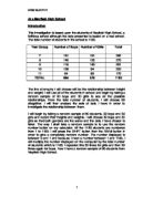
I will begin testing this hypothesis, by taking samples of 28 boys from year groups 7 and 10. I will take these samples by using the random number generator in Microsoft Excel again.
After I have selected my samples, I will illustrate the data in tables, by year group, therefore making it easier to use and interpret the data. Then I will use the data to create a line graph. The line graph will contain both sets of data, from both year groups. Therefore it will be easier to compare the two sets of data.
I think that this will be the best method as:
They are good at showing specific values of data, meaning that given one variable the other can easily be determined.
They show trends in data clearly, meaning that they visibly show how one variable affects the other as it increases or decreases.
They enable the viewer to make predictions and interpretations easily.
5. The girls’ growth spurt is greater than the boys’ growth spurt.
In order to investigate my hypothesis above, I will take samples of 28 boys and girls from year 7 and 28 boys and girls from year 10. This will be achieved by using a random number generator in Microsoft Excel.
After I have got my samples of pupils, I will use a frequency polygon to illustrate the data.
I will have one frequency polygon for boys, and one frequency polygon for girls, with both year 10s and year 7s of each gender plotted on the same graph. This will also make the data easier to interpret. When I have plotted the graph, I will use the results to see whether girls really do have their growth spurt earlier than boys.
I believe that frequency polygons would be the best method to use, as it will be easier to compare and interpret the distributions.
Anomalies
I am aware that I may select some anomalies, in these circumstances, I will compensate by selecting another pupil at random.
Method
1. There is a weak positive correlation between height and weight between girls and boys at Mayfield High School.
I started investigating my first hypothesis by taking my stratified samples, using Microsoft Excel.
Boys
Girls
Having taken my stratified sample, I used to the random number generator to choose the pupils for sampling. First I took the year 7 pupils from the database and then I sorted them into order by gender, by highlighting them and using sort in the Data toolbar. Once they were sorted out by gender, I numbered the pupils the boys and girls. The girls were numbered from 1 to 131 and the boys from 1 to 151. Next I highlighted all of the boys and, using the formula =RAND()*151 (151 is the total number of boys in year 7) selected 6 numbers at random between 1 and 151.
Although, initially I got numbers with many decimal places but I changed this to numbers without any decimal places, in order to get whole numbers all the time. This was done by highlighting the cell with the decimal places and going to the Format Menu and then into the Cells Menu. Here I changed the number of decimal places. I then got whole numbers only, these numbers were:
I used the same method for both genders in each year group from year 7 to year 11, and selected the correct number of pupils from each year group according to the numbers shown in the stratified sample tables above.
Year 7 Boys
Year 7 Girls
They were numbered from 1 to 127.
Year 8 Boys
They were numbered from 1 to 146.
For my 6th sample initially, I got random number 67, the pupil called John Hall, who appeared to have a weight of only 5kg. I assumed that this was an anomaly and replaced it with another randomly generated number. This was number 127, the pupil Jonathan Thomas.
Year 8 Girls
They were numbered from 1 to 124.
Year 9 Boys
They were numbered from 1 to 118.
Year 9 Girls
They were numbered from 1 to 143.
Year 10 Boys
They were numbered from 1 to 104.
Year 10 Girls
They were numbered from 1 to 94.
Year 11 Boys
They were numbered from 1 to 84.
Year 11 Girls
They were numbered from 1 to 84.
Having taken all of my samples, from the students, I took all of the heights and weights of the boys and all of the heights and weights of the girls, and plotted them on a scatter graph, to see whether there was a weak positive correlation between the boys and girls.
I did this by taking the heights and weights of the boys and girls from the tables above and sorting them into two columns for by gender.
Next I highlighted all of the data and went to the table wizard. Here I chose the XY Scatter Graph option and in the ‘Series’ menu chose to distinguish the data of the girls from the boys. As they already had all the information about the boys in ‘Series 1,’ I added another Series and labelled it ‘Girls’.
I highlighted all of the figures for the weights of the girls and put them into the ‘X values’ and highlighted all of the heights of the girls under ‘Y Values’.
Then I labelled both axis in the ‘Chart Options’ menu and then clicked the ‘Next’ and ‘Finish’ buttons to generate my graph.
Scatter Graph: Correlation between Heights and Weights amongst Boys and Girls at Mayfield High School
To see whether there was any correlation between the heights and weights of boys and girls in Mayfield High School, I used the product moment correlation coefficient. I did this by right clicking on each trend line on the graph and displaying R squared (as seen above). Having done this, I square rooted R squared to get a decimal number between –1 and 1. The scale goes as follows:
-1 0 1
-1 means that there is a strong negative correlation, 0 means that there is no correlation and 1 means that there is a strong positive correlation.
The PMCC for the boys in Mayfield High School was:
R squared = 0.3703, therefore
R = 0.6085 (to 4 decimal places).
This shows that there was a fairly strong, positive correlation between the heights and weights of the boy.
The PMCC for girls in Mayfield High School was:
R squared = 0.099, therefore
R = 0.3146 (to 4 decimal places).
Interpretation
Looking at the graph, I saw that the correlation between the heights and weights of the boys was fairly strong and positive; this was confirmed by the value of R, which was 0.6085.
On first impressions, I thought that the correlation of the height and weight for the girls was fairly weak and positive. These thoughts were confirmed by the value of R for the girls’ correlation.
2. The spread of data for height between the lower and upper quartiles will be greater amongst yr11 girls compared to yr 7 girls.
I started investigating the hypothesis above by first taking 28 female students from year 7 and 28 female students from year 11 to use as my samples.
I did this by going to the Mayfield High School database and extracting the year 7 and 11 girls, by copying them into a new document, numbering them, depending on how many there were in each year group, and then using the Rand between method in Excel to generate 28 random numbers.
I had to choose many sets of numbers as the same number came up twice many times, but once I had chosen 28 different numbers, I selecting the 28 pupils that had been chosen. Although before this I used the ‘Format Cells’ menu to change the number of decimal places to 0, in order to get whole numbers only.
Below is a table showing which year 7 girls were chosen at random.
Initially for sample number 9, I got a student weighing 110kg, about three times as much as the other students. Therefore I concluded that she was an anomaly and randomly chose another number, in order to get another student.
Below is a table showing which year 11 girls were chosen at random from 84 pupils.
Having obtained all of the data about the pupils I was testing, I took the heights and used graph paper to construct my box plots. Although, before this, stem and leaf diagrams were drawn. This was to sort the data into order and to find out the values of the quartiles.
Stem and Leaf diagram for the heights of pupils in year 7
1.2 5
1.3 2, 2
1.4 3, 6, 8, 8
1.5 2, 3, 3, 4, 5, 6, 6, 7, 9
1.6 0, 1, 2, 2, 2, 2, 3, 3, 3, 5, 5
1.7 5
Using the diagram above, I found the values of the quartiles to be:
Q1 = 1.50
Q2 = 1.565
Q3 = 1.62
The Stem and Leaf diagram below shows the heights of the 28 year 11 girls that were sampled.
1.3 7
1.4
1.5 2, 2, 5, 6, 6, 6, 8
1.6 0, 0, 1, 2, 3, 3, 3, 5, 5, 5, 5,
1.7 0, 2, 2, 2, 3, 3
- 3
Using the stem and leaf diagram, I found out that the values of the quartiles were:
Q1 = 1.57
Q2 = 1.63
Q3 = 1.72
Using the values of the quartiles that I found using the stem and leaf diagrams, I plotted the box plots. I drew both of them on the same scale, which made them easier to compare with one another. (See appendix 1)
Interpretation
Having plotted the box plots, I found that the box plots of the year 7 girls was not skewed heavily towards either quartile, the data was roughly evenly spread between Q1 and Q3.
However, the data between the upper and lower quartiles in the box plot of the year 11 girls was skewed towards Q1. This shows that the heights are clustered between the median and where as the heights between the median and Q3 are more spread out.
I also noticed that the year 7 girls have a wider range of data compared to the year 11 girls.
3. There is a higher concentration of closely related BMIs for boys in year 8 compared to boys in year 11.
I began testing this hypothesis by taking 28 random samples of boys in either year group, using Microsoft Excel, and the Rand between function again. I extracted the heights and weights of each pupil, and the used this formula to find out the Body Mass Index of each pupil:
BMI = Weight (in kilograms) / [Height (in metres)] * [Height (in metres)]
I rounded the values of the BMIs down to 2 significant figures, to make it simple and easier to read and interpret.
The table below shows the data that I collected from the boys in year 8.
The table below sows the data I collected from my sampling of the male students in year11.
I used the BMI column to plot histograms on graph paper. Although before this, I sorted the data into ascending order and drew up a frequency tables, as shown below. I included a frequency density column. This is found using the formula:
Frequency Density = frequency / class width
All of the frequency density values were written to 1 decimal place.
This is a frequency table classifying the data for the year 8 boys.
This is the frequency density table classifying the data of the year 11 boys.
Using the tables above, I plotted two histograms, using the same scale for both, making it easier to interpret and understand.
Interpretation
Having looked at each histogram, I thought that there was a higher concentration of closely related BMIs in year 11. I determined this, as the frequency density total for the year 11 boys is greater.
In general, the area the histogram for the year 11 boys was greater, therefore meaning that the concentration of closely related BMIs is higher.
4. The older the boy the heavier he is.
I again started testing this hypothesis by taking 28 random samples. The random samples were taken of boys in year 7 and boys in year 10. The same method for the random number generator was used, just as it was used in the other hypothesis.
In the table below the data I extracted from the database is shown. It shows the pupils that were selected at random from year 7, with their weights.
The table below also shows the randomly chosen pupils from year 10 and their weights.
Having taken all of my samples, I took the heights from the tables and plotted the line graph, using the table wizard in Microsoft Excel, with both sets of data on the same graph.
A Line Graph showing the weights of boys in year 7 and boys in year 10
Interpretation
The line graph above clearly shows that the older the boy is the heavier he is. Almost all of the year 10 boys are heavier than the boys in year 7, with only one or two exceptions.
5. The girls’ growth spurt is greater than the boys’ growth spurt.
In order to investigate my final hypothesis, I took 28 random samples of boys and girls in year groups 7 and 10. Again I used the random number generator, to select my random numbers, and then I used them to select the students and their weights.
A table showing the heights of girls in year 7 is shown below.
A table showing the heights of the boys selected from year 7 is shown below.
A table showing the heights of year 10 boys is shown below.
A table showing the girls selected and their heights is shown below.
Having selected all of the students for testing, I took the data for each year group into excel and used to create a frequency polygon.
Graph showing the height of girls and boys from year 7 and year 11
The graph above shows that the boys do in fact have a greater growth spurt than girls. This is shown as the area between the lines showing the heights of the boys are greater than those of the girls.
Conclusion
Overall, having drawn interpretations for each hypothesis individually, I think that in some categories there was a trend as you went up the school. For example, the line graph for my fourth hypothesis shows that as the boys got older their weights increased steadily with their age, with only a few exceptions.
I also noticed this trend with the graph I drew with in hypothesis five. Both boys and girls’ heights increased steadily with age, with only a few outliers who did not grow that much.
However these results could have been affected by the size of the sample. The samples were only a small representative value for each year group. Unseen anomalies could have occurred through people with conditions that I may not have picked up. My data may not have been totally accurate, as I may have selected the same people many times for my sampling.
Also with some of my results, I noticed that as the students got older, they seemed to all be in the same height and weight categories. This is shown particularly in the hypothesis I did on Body Mass Index. The outlying class widths seemed to disappear and move towards the main class widths in the centre. This effect was also shown in the box plots that I plotted. The difference between the ranges decreased dramatically with age.
I believe I did this coursework quite accurately as I did take into account and compensate for most anomalies, and other outliers in the database. Although, I may not have taken a sufficient number of people to sample, or have taken into account anomalies that could have gone unnoticed in the database.